This page was created in response to requests from readers of the articles on this site reviewing many aspects of TTC surface operations:

• Over time, I have become so used to publishing these articles that I tend to forget that people who come to them don’t just say “oh, but of course that’s what he is doing here”. There are lots of (mostly) pretty charts, but what do they mean?
• On occasion, I get requests for more detail via comments, emails, or social media messages, but the sheer volume of material makes replies challenging.
• There is already an article describing the mechanics behind creation of these charts (see Methodology For Analysis of TTC’s Vehicle Tracking Data), but it is intended for the technically inclined who want to know how the TTC data are transformed.

I chose to structure this primer from the details outward to the consolidated view of data. Going at it the other way presents the challenge of showing summaries which beg the question of “but where did that come from” rather like trying to describe a forest before explaining what trees are.

Each section of this article deals with one type of chart so that you can skip to the portion of interest if that’s your preference using the links below:

• Daily “as operated” service charts
• Daily headway and link time charts
• Monthly headway and link time charts and histories
• Travel time histories
• Speed charts
• Service capacity charts
• TTC service quality metrics

What Was The Inspiration For This?

Over the decades of my activism for better transit, and especially for the recognition of the role streetcars can play both in mixed traffic and in an LRT (“Light Rapid Transit”) setting, there are persistent claims that “buses are better”. Without doubt, there are places this is true, but I wanted to understand how real live transit service actually behaves.

This began in 2007 with data from the rather primitive tracking system used by the TTC which had a major limitation: it didn’t track vehicles particularly well. The situation improved in 2010 with the introduction of GPS tracking so that a vehicle’s location was more-or-less accurately known most of the time. (For a detailed description of the peculiarities of the tracking systems, please see the “Methodology” article.)

Back in 1985, Vancouver opened its SkyTrain system. Whatever arguments I might have about the technology, I was impressed with an important line management tool when I visited their control centre. From the first day of operation, they produced charts showing how the service actually behaved. Even though it was fully automated, the system still depended on manual supervision to “tweak” service and select operating strategies. Sometimes this worked, and other times, service could be a shambles.

The charts allowed a review of the line’s actual behaviour under many conditions. How reliable was the service? Were tactics to rearrange service actually working? Were there constraints in the operating plan?

At that point, the TTC’s original tracking system, CIS, did not yet exist. It would be another two decades until I began to receive data extracts from it. These quickly revealed what riders knew all too well — service on surface routes generally, not just streetcar lines, did not operate anywhere near its advertised schedule reliability, and this was not, as the TTC fondly claimed, entirely the fault of “congestion”.

All of the work since then on improving and expanding the repertoire of charts of TTC service have concentrated on making visible the behaviour of routes seen as a whole, not from the limited vantage of a rider standing on a windswept street corner wondering if their bus will ever arrive.

“As Operated” Daily Service Charts

The first type of chart I set out to build was a graphic representation of actual, as opposed to theoretical, operations, and this was directly inspired by what I had seen in Vancouver.

The idea of representing operations of a transit or railway line this way is not new, and it dates back to the 1840s when it was created by a French engineer, Charles Ibry. There is a wonderful article, From Paris With Love, about this on Sandra Rendgen’s website (with historic illustrations!) that is very much worth a visit.

If one plots TTC service the way it is scheduled, the chart is interesting because it shows that ideal service we never, ever see. This is the afternoon peak period for the schedule that took effect on June 22, 2020. The service is quite mundane with regularly spaced cars, but it will do as an introduction.

For this type of chart, a route is treated as a straight line even though in practice it twists and turns. In effect it is as if a route on a map were a piece of string that one picked up and stretched out straight. (The process of converting from the meanderings of real geography to a one-dimensional version is explained in the “Methodology” article.)

Thinking of a route as a line starting at “zero” (typically just beyond one of the termini) and running to an upper value depending on the length of the route. The GPS positions in tracking data are translated to 10 metre increments along the route (roughly a standard bus length). This is small enough to resolve intersection geometry (nearside and farside stop locations) without requiring a very large range for most routes. (There is little point in trying to be too accurate thanks to the vagaries of GPS position data.)

Distance runs from east to west, bottom to top, with Neville Loop at the bottom and Long Branch up at the top. Various intermediate streets lie in between. Because this is the schedule, all of the lines run the entire distance from one end of the line to the other.

Time runs across the bottom starting at “16:00:00” or 4 PM going to 7 PM. A PDF with the full day’s schedule is linked below.

Lines sloping upward represent westbound cars, and those sloping down are eastbound. The times and locations are based on the schedule which is published in a standard format (“GTFS” or General Transit Feed Specification) by the TTC for each new schedule period.

The slope of the line indicates the scheduled speed. The more vertical the slope, the shorter the travel time and hence a faster speed. If a line were horizontal, this would represent a stopped car.

The space between the lines is the “headway” or time between cars. The closer the lines, the more frequent the service. On this schedule, a standard 10-minute frequency is scheduled, and the lines are all the same space apart.

By contrast, here is the real service operated on 501 Queen during the afternoon peak on Monday, June 22, 2020. Many facets of real world operation are visible here.

• The small wrinkles in the lines represent places where a car stopped enroute. At terminals and a few other locations the pauses are longer and they show up as an extended horizontal line.
• The uneven headway is visible in the spacing of the lines.
• A diversion between Broadview and Parliament shows up as a break in the chart because the “map” I used to plot service only includes the standard portion of the route. The shuttle bus shows up making a round trip across the gap now and then with siestas between each trip.
• A few short turns at Woodbine Loop (between Coxwell and Woodbine) and at Russell Carhouse (east of Greenwood) as lines that run horizontal for a time, then go back westbound without reaching Neville Loop.
• There is little difference in the slope of the lines, except to a small degree between Roncesvalles and Humber, because the covid-era traffic does not produce any congestion to speak of.

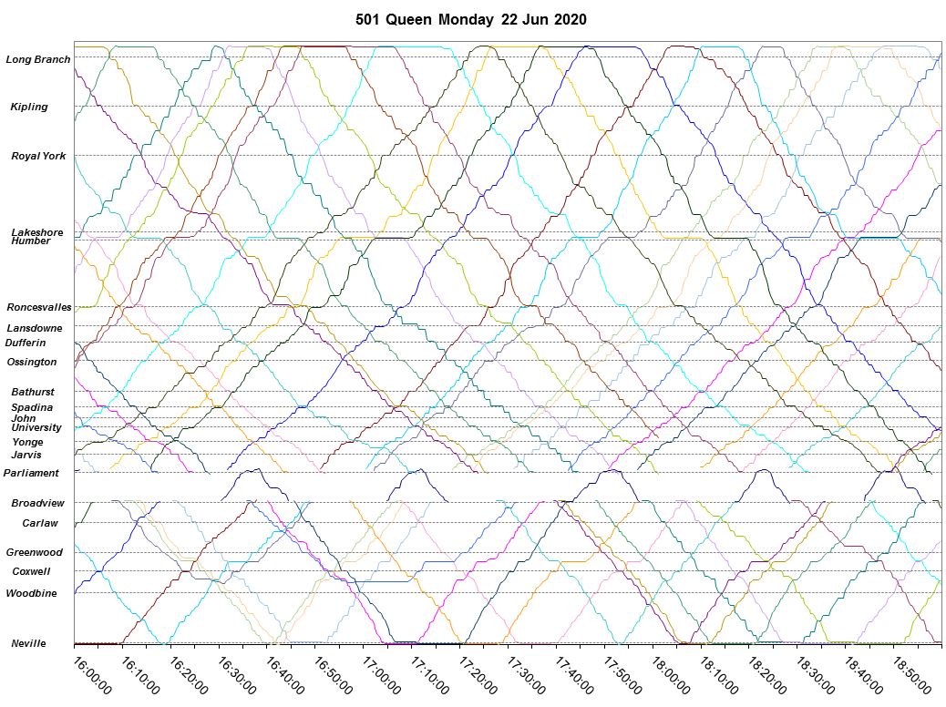
The full set of charts for June 22, 2020 is linked below.

By comparison, here is the service on Tuesday, June 18, 2019 under more “classic” traffic conditions for the AM and PM peak periods. Note that at the time this route operated with CLRVs and more frequent scheduled service than in 2020 with Flexitys.

Among the issues visible here are:

• Congestion both ways between Spadina and Yonge, and approaching Lansdowne is visible with lines that run more horizontally than in other parts of the chart.
• The separate operation of the Long Branch portion of the route is visible with cars that only run between Humber and Long Branch, with a few turning back at Kipling.
• There are short turns at Greenwood and at Woodbine Loop in the east end, as well as at Roncesvalles in the west.
• Irregular headways and bunching show up quite clearly with some lines (pairs or triplets of cars) running close together for an extended distance.
• During certain periods, cars “disappear” in the Beach before they reach Neville, and the reappear on their westbound trips. This is not a GPS problem, but rather a side-effect of operational procedures where operators “sign off” the tracking system before reaching the terminal. This affects calculations of headways near Neville (see below).

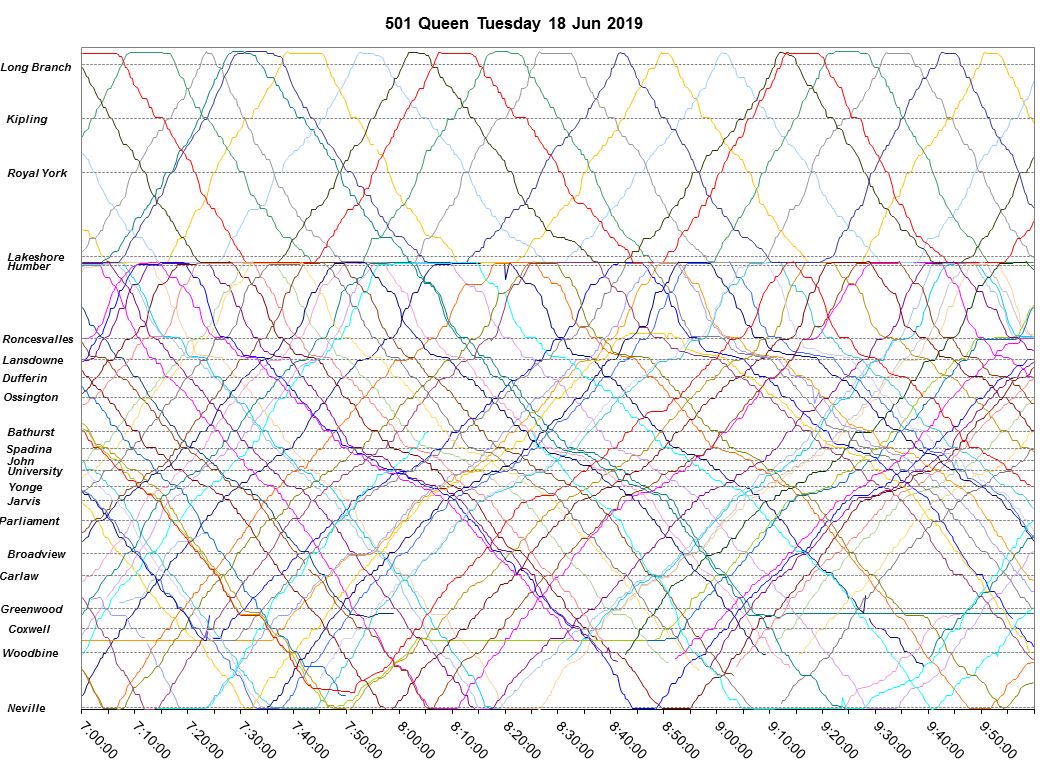
The full chart set for June 18, 2020 is linked below.

A Special Case: Branching Routes

Some routes have a branching structure and this does not fit directly with the “stretched piece of string” analogy used earlier. Instead, a route might have a “Y” structure with a common inner end and two or more outer branches, or it could have a “Y” at both ends.

70 O’Connor is a simple example of the “Y” arrangement with a common southern terminus at Coxwell Station, but two separate northern branches to Warden Station and to Eglinton. These are handled by, in effect, “cutting the string” so that one branch of the “Y” is looped off from the other.

In this chart, the segment from St. Clair to north of Eglinton is split apart. Northbound buses disappear at the “St. Clair” line in the lower part of the chart, and reappear in the upper section, with a similar effect on the southbound trip. This chart shows a particularly bad day on the O’Connor bus with much bunching, a topic covered in separate articles.

Buses clearly leave terminals in a bunch and travel together over the route leaving wide gaps in service. There is no evidence that anyone attempts to space the service to correct this problem. The TTC claims that there were untracked extras operating, but they have not provided any evidence of this. In any event, the chart shows that service does not operate on anything resembling a regular headway for several hours.

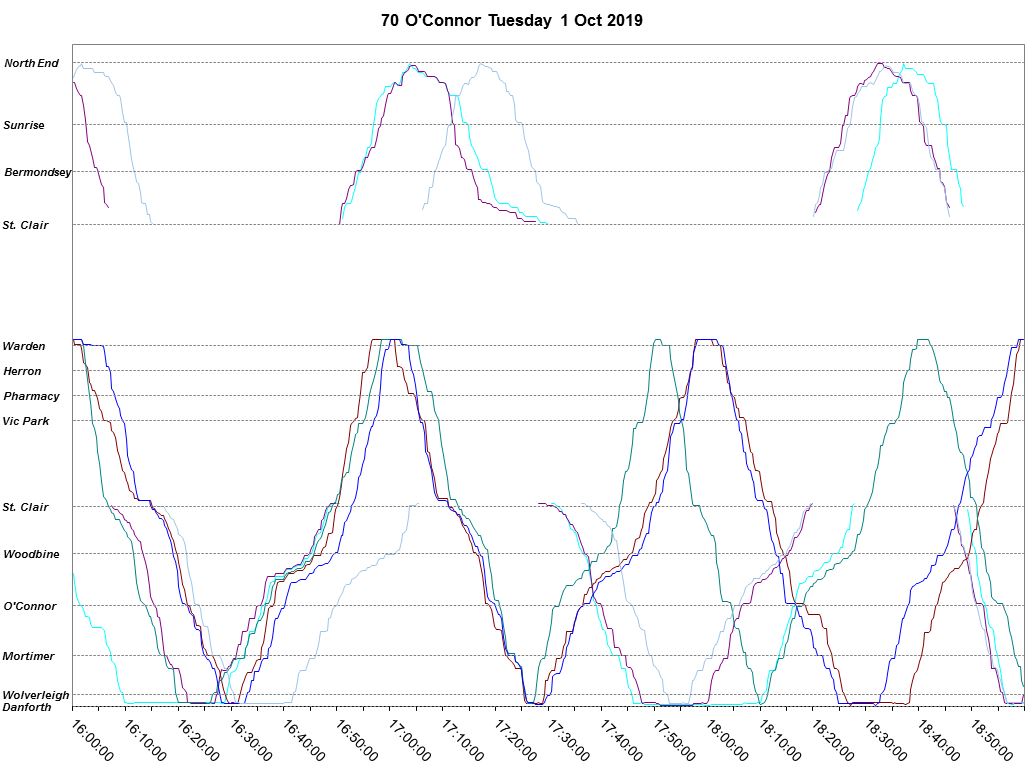
The full day chart is linked here.

An example of route with branches at both ends is the 504 King streetcar which has two eastern termini (Broadview Station and Distillery Loop) and two western (Dundas West Station and Dufferin Loop). In this case, the two relatively short branches are lopped off to leave the main route as one continuous piece with the Distillery and Dufferin branches off by themselves.

The short segment between King and Dufferin Loop appears at the top of the chart while the short Cherry Street section to Distillery Loop is at the bottom. The lines are more closely spaced in the central section of the chart where the 504A and 504B services overlap.

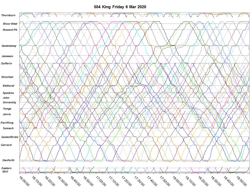
The full day’s charts are linked below.

These charts establish what the service looks like overall, but we need to view the data in different ways to tease out other useful information. One thing will be quickly apparent to readers — there is a lot of detail here just for one day, let alone for weeks of operation by multiple routes. In the sections after this, I will turn to various forms of consolidation to look at the larger patterns.

Although it is important to not be overwhelmed by the details, it is also important to know that at a fine-grained level the data look a lot different from the result one gets from summaries and averages that mask what is really happening.

Daily Headway and Link Time Charts

Time Points and Screen Lines

To review the service at a fine-grained level, we need to know when vehicles pass specific points along the route.

• The time between vehicles passing is the headway, the time interval between them.
• The time between a vehicle passing point “A” and point “B” is the travel or “link” time between the points.

For these analyses, the “map” of a route contains specific “time points” which are of interest. These have been set up when I first defined the maps to capture a reasonable set of locations where and between which measurements might be of interest. They are included on the daily service charts as horizontal reference lines (see samples above).

With very rare exceptions, these have stayed the same through many years of service analyses to allow direct comparisons and production of charts showing how service evolved.

Note that these time points are not the same as those used in TTC schedules. They are defined to break routes into segments of interest for my analysis. Moreover, TTC schedule time points refer to arrival and departures at stops, while the screen lines (see below) are defined in the middle of intersections, not at the stops.

Traffic engineers use the term “screen line” to define a place where there is an imaginary line across one or more roads where traffic volumes are measured. In my analyses, I establish screen lines at or near the time points with the same intent, although there are a few wrinkles worth noting.

• For a screen line at an intersection, this is defined in the middle of the intersection so that stopping positions, be they nearside or farside, are not split by the line. This avoids problems with defining different screen lines for each direction of travel to deal with stop placement.
• For a screen line near a terminal, the location is chosen a short distance away to allow for vehicle congestion and queuing at the terminal. If the screen line is defined right at a terminal, this queuing time can erroneously be counted as travel time rather than as terminal time.
• For special, fine-grained analyses, closely-spaced screen lines can be used to distinguish movements between stops and within the stopping area. For example, the 512 St. Clair car has most stops on the far side of intersections, but there can be interference between traffic signals and streetcars that holds them on the nearside. This can be analyzed by treating the nearside approach to an intersection, the crossing itself, and the farside car stop as three separate “mini links” to determine where streetcars are spending their time.

As a prelude to creating the headway and link time charts, the data from the daily service charts are converted to “as operated” schedules. These are not published in the articles, but they directly generate the charts. They are, in effect, what a timetable would look like if it reflected the service as actually experienced on the street. Headways and link times can easily be calculated from this information.

Daily Headway Charts

501 Queen is complex route where service is often disrupted. However, the western portion between Humber and Long Branch was better behaved when it operated as a shuttle. This shows a typical pattern for a simple route.

The common message here is that there is a huge difference between service as measured at terminals versus along the route. Looking at the “average” level of service hides the constant effects of gaps and bunching, some of which originates from terminals and worsens as vehicles travel along their route.

Although the charts here are for 501 Queen, the patterns seen here show up across the network with both bus and streetcar routes including those operating in reserved lanes.

More riders are affected by a wide headway than a narrow one because they accumulate for a longer period. The total waiting time varies with the square of the headway. If the headway is double what it should be, twice as many people will be waiting when a car arrives, and they will wait on average twice as long for a car. Hence four times the total “wait minutes”.

Similarly, a “gap car” will be crowded while its follower will be lightly loaded. There are more riders on the crowded cars, and that is what most riders experience. Complaints about packed vehicles rarely line up with management statistics based on average loads measured over many vehicles.

June 18, 2019

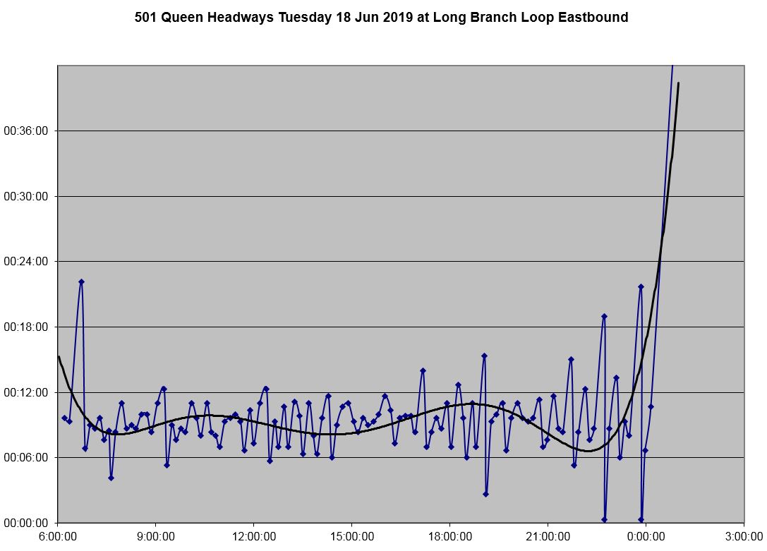
The chart below shows one day’s operation eastbound crossing the screen line just east of Long Branch Loop. This shows actual headways varying over a range of about six minutes. Each dot represents one car. The black line shows the overall trend in values through the day. This shows how riders see irregular service even though a report of “average” headways would not reveal any problems.

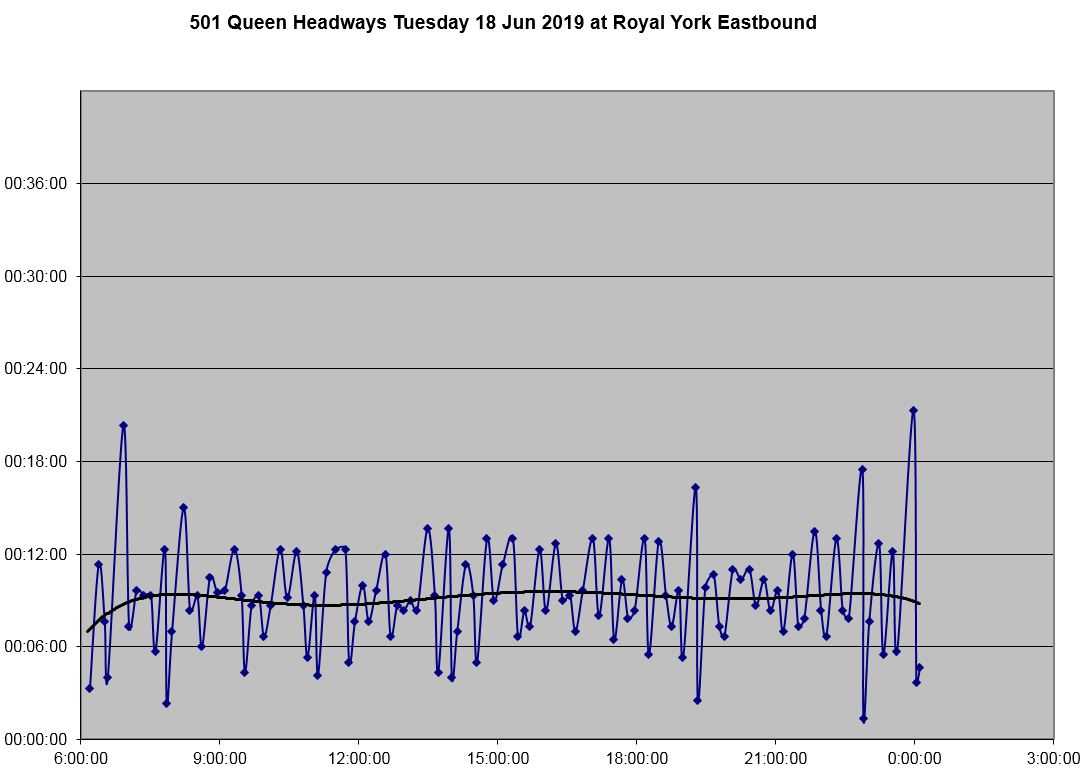
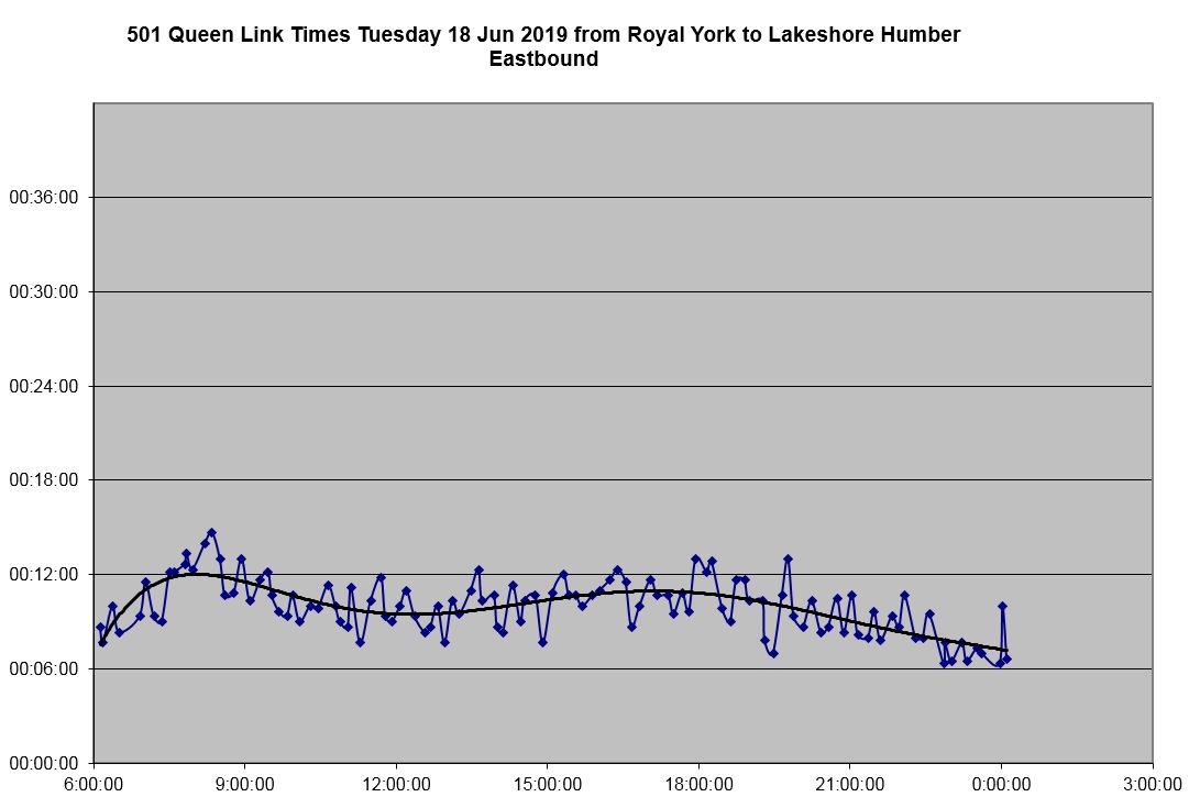
By the time this service reaches Royal York, the swings in headways have widened. This is typical for all services because vehicles running in wider gaps are delayed more at stops, while those in short gaps have a faster trip and catch up to their leaders.

Again, the trend line shows a stable service level through the day, but this masks the variation in individual trips.

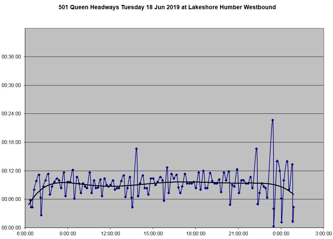
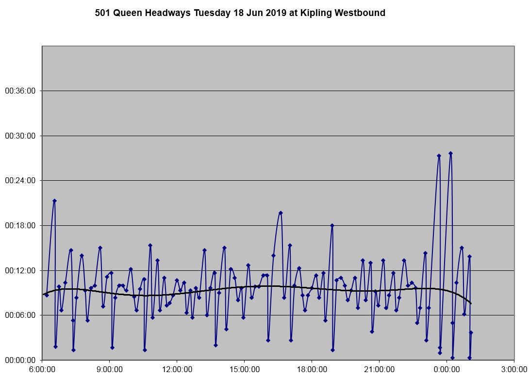
The situation westbound is similar. Service leaving Humber Loop westbound lies within a six minute band for much of the day, but is much less regular by the time it reaches Kipling Avenue. Again, the trend lines give no indication of the swing in actual headway values.

On the main part of the Queen route, service was more frequent in mid-2019, but also more erratic.

Leaving Humber Loop eastbound, service is erratic almost all day long. Many cars leave on very short headways, and there are two notable service gaps just before noon and at about 3 PM.

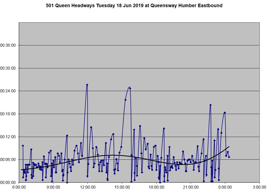
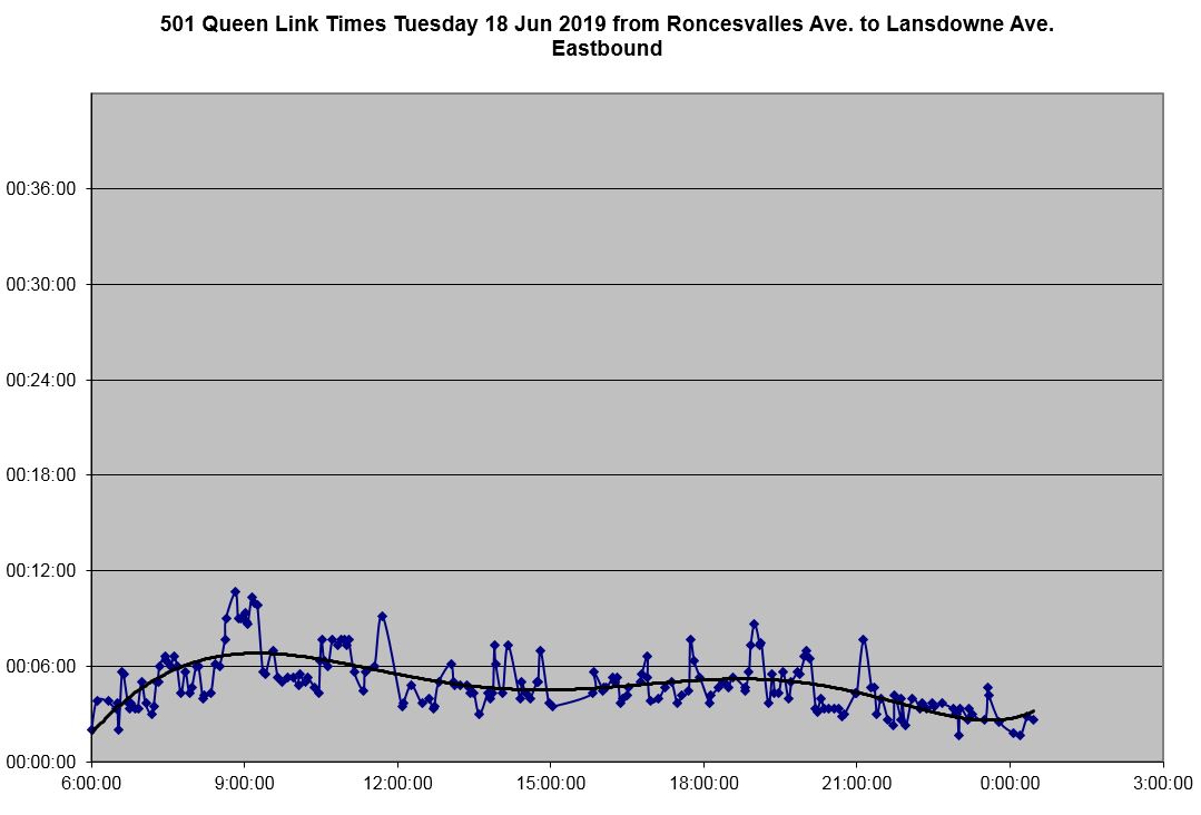
At Roncesvalles, the two large gaps persist indicating that nothing was short turned here to fill them. The short headways are generally not at the zero line because the nature of this intersection is such that two cars rarely cross on the same signal cycle, and pairs are separated, slightly compared to departures at Humber.

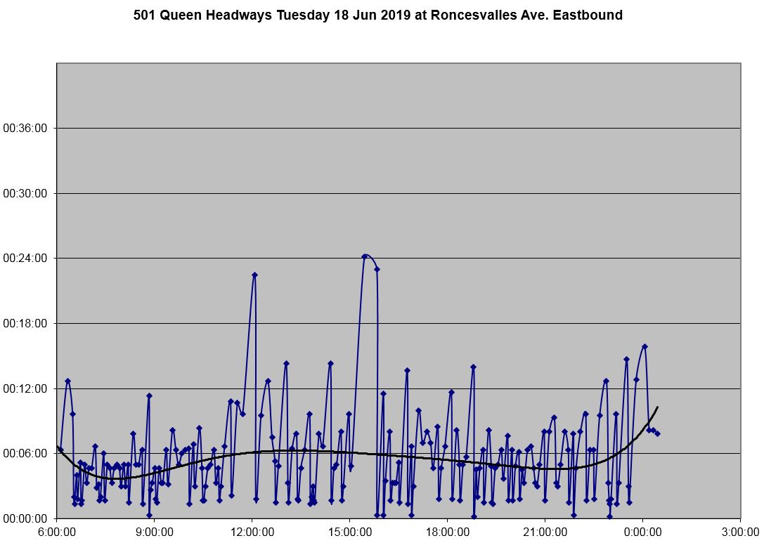
At Bathurst Street, the mid-day gap has been filled by a short turn, but the mid-afternoon gap remains. The range of headways is now well above a six-minute window with many cars running in pairs followed by 15 minute or greater gaps.

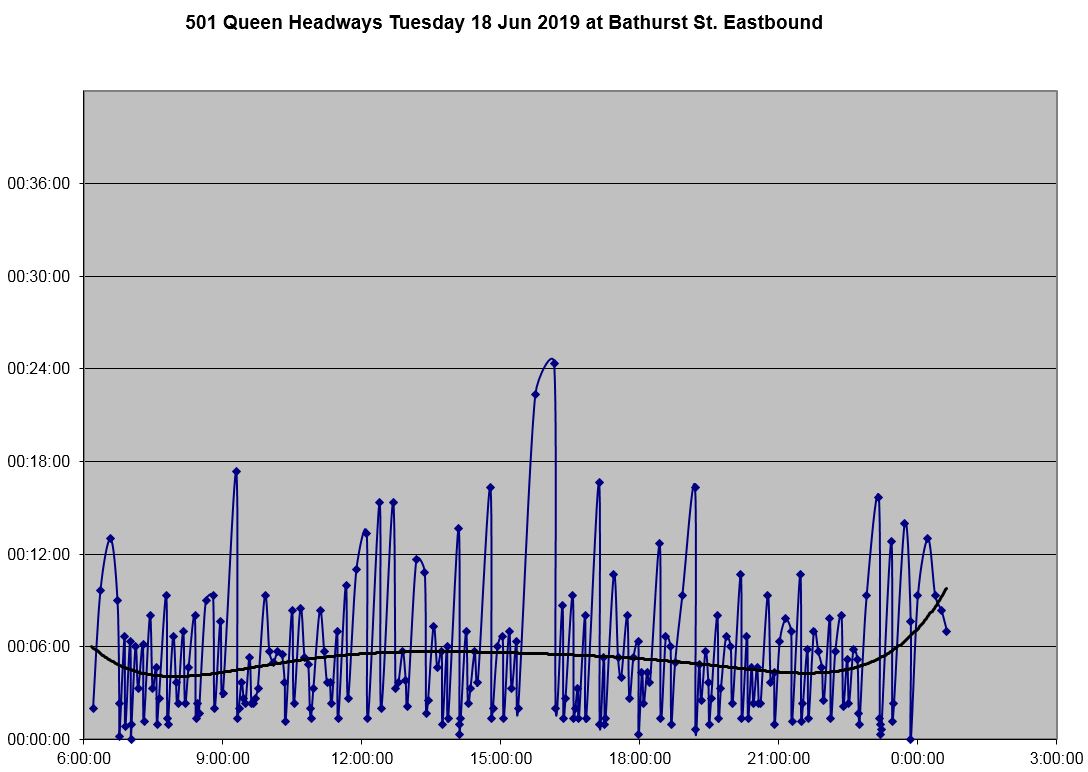
At Yonge Street, the situation is the same as seen at Bathurst.

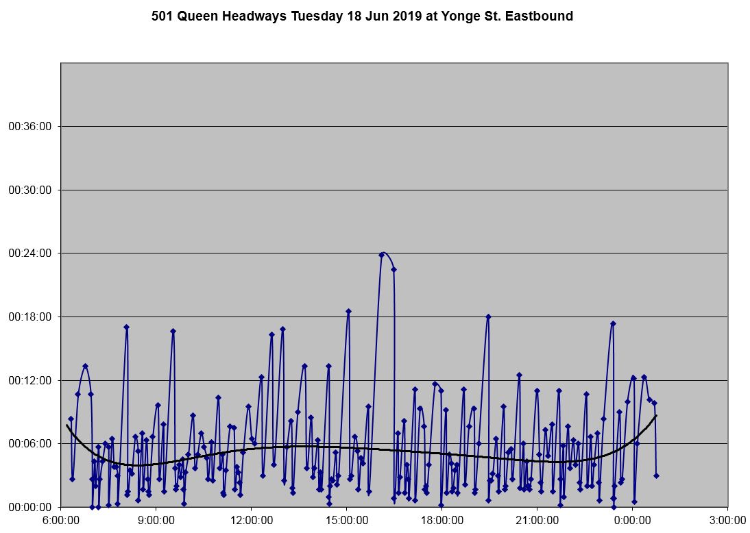
At Woodbine Avenue, the range of headways continues to widen with longer gaps especially in the afternoon and evening. Many of these gaps did not exist at Yonge Street indicating that short turns prevented all of the service from reaching the Beach, compounding the gaps caused by bunching.

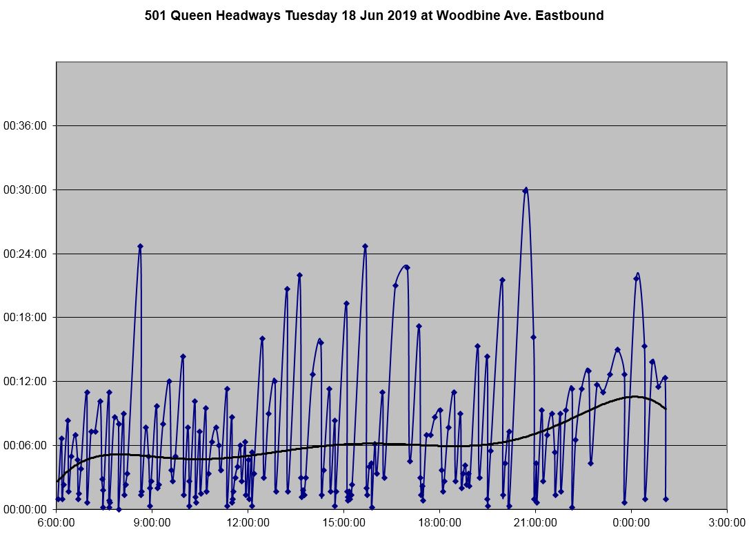
I have not included the chart for Neville Loop because of the problem of “disappearing” cars noted earlier.

The full sets of charts for each direction’s operation are linked below.

Christmas Day, 2019

As an example of how the tendency to bunch is almost inevitable, here are the headways on Queen on Christmas Day, 2019.

Leaving Humber Loop eastbound, daytime headways are fairly well behaved, but there are occasional cars running close on the tail of their leaders.

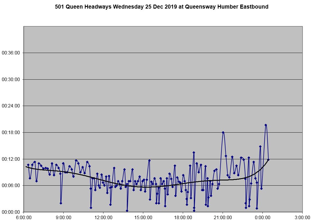
By the time this service reaches Yonge Street, the swings in headways are more pronounced.

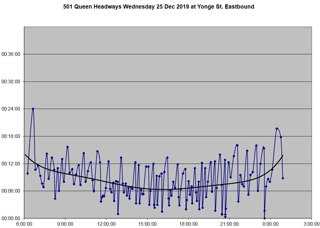
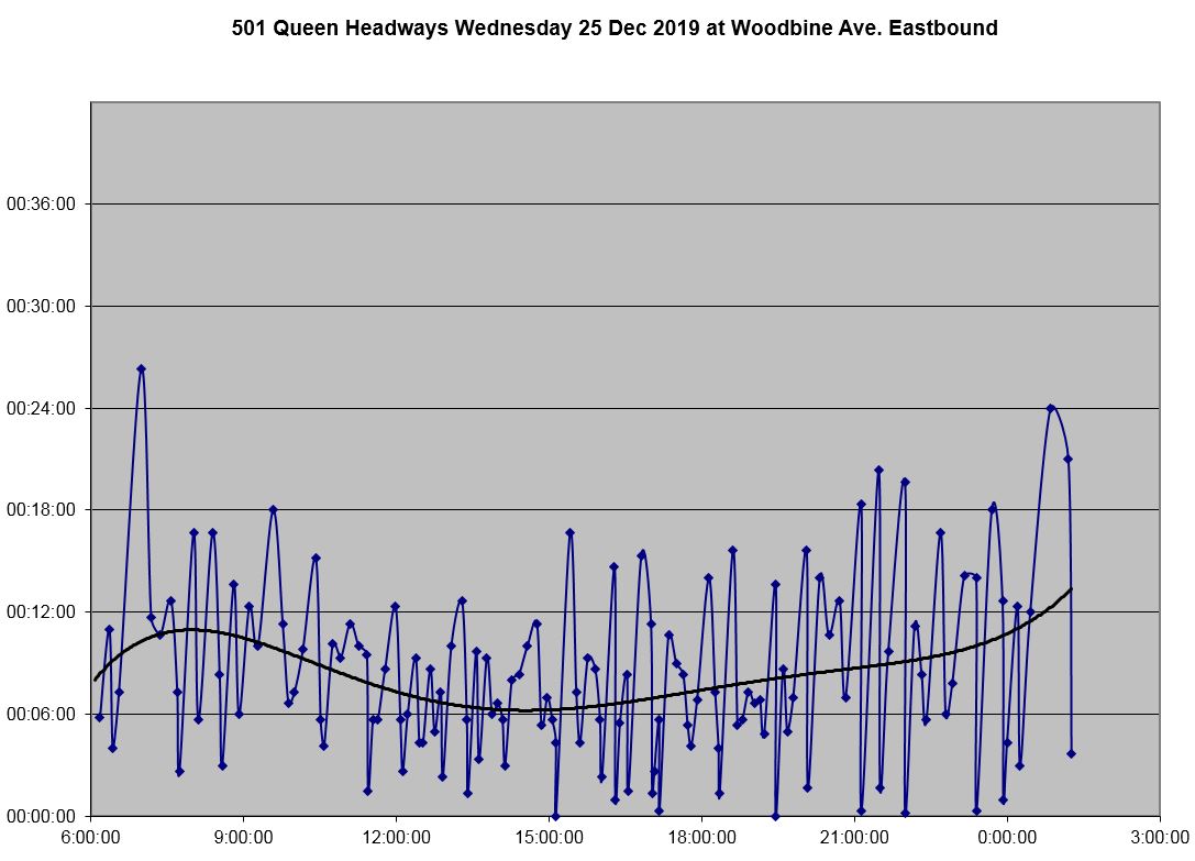
At Woodbine, the situation is even worse. Even though the service began with a well-regulated headway in the west end, by the time it reached the east end there were more bunches (short headways) and wider gaps (long headways).

The situation westbound was no different. Here is the service westbound one stop west of Neville Loop. Headways stay in a narrow band with few exceptions through much of the day.

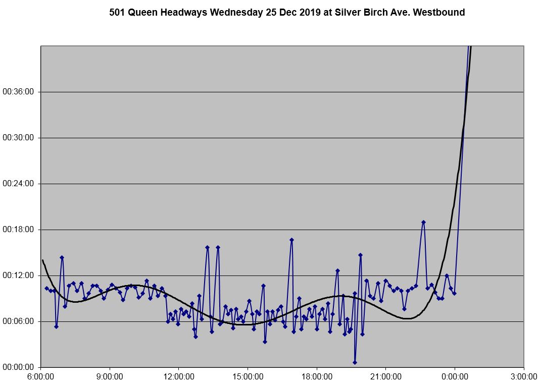
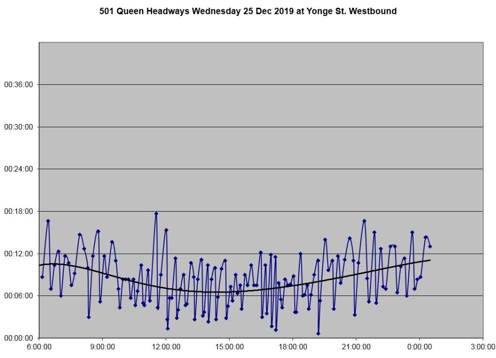
By the time the service reaches Yonge Street, things have changed and headways are irregular, alternating between roughly 2 and 12 minutes.

Westbound at Roncesvalles, including service through the evening, cars are commonly running in pair or close behind each other.

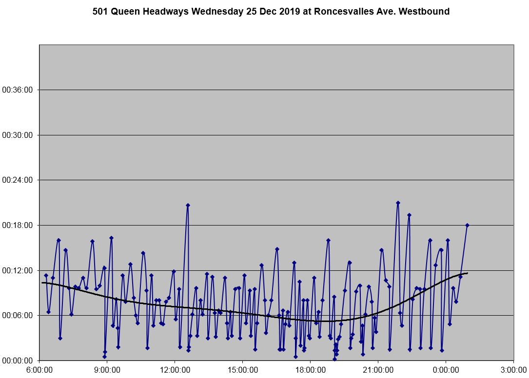
Through all of this, the trend lines are quite smooth and the averages would give someone the impression that the service is quite good when in fact longer than scheduled waits would be common.

Here are the full sets of charts for Christmas Day headways along the Queen route.

Daily Link Time Charts

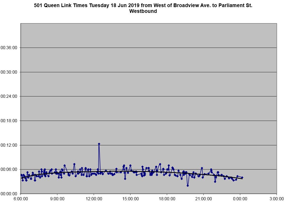
Link time charts show the travel time between the time points on a route. They have the same format as the headway charts, but they convey different information. This section includes samples for the Queen car from June 18, 2019, the same day as the headway charts in the previous section.

By splitting the route into smaller segments with screen lines, the effect over each segment can be seen clearly. This is important for reviews of potential transit priority schemes to identify locations where there is actually something to gain. No route is congested all of the time over all of its length. With competition for road space among motorists, delivery vehicles, cyclists, pedestrians and transit, we must know where the key potential benefits lie.

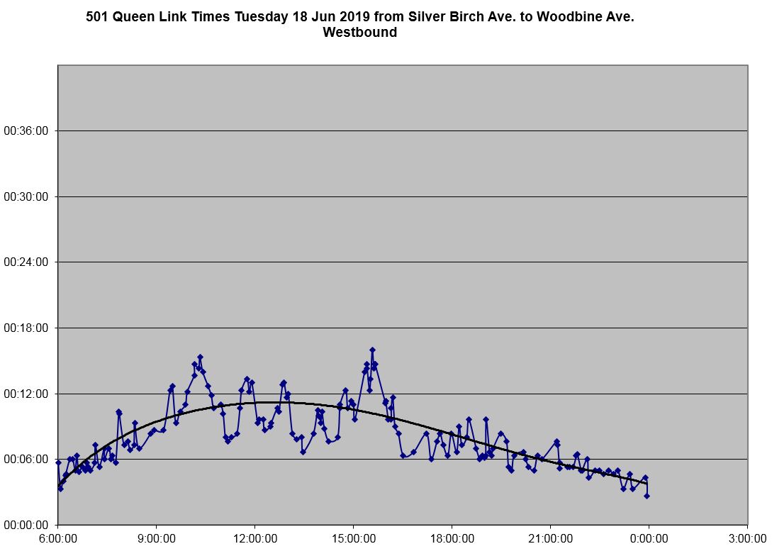
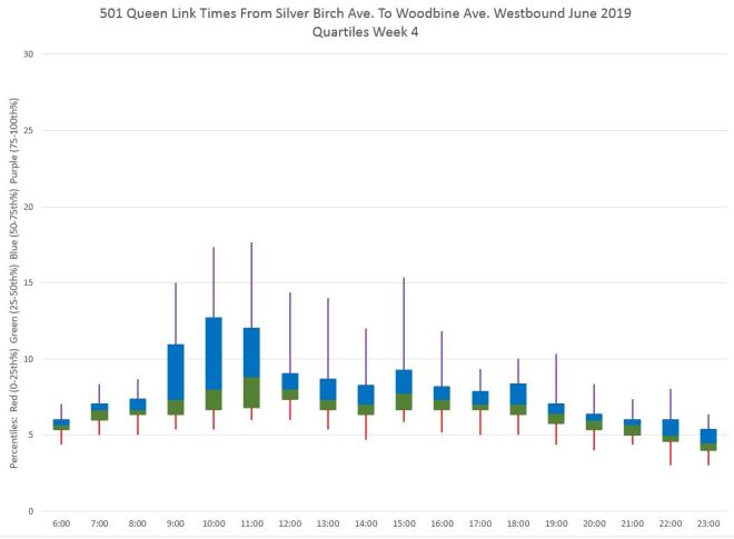
Here are the travel times westbound from Silver Birch (the first stop west of Neville) to Woodbine. Note that the longest travel times are between the peak periods. A fairly common pattern is for there to be longer times just after the AM peak and just before the PM peak because off-peak parking rules kick in reducing the street’s capacity while there is still heavier traffic. There have been adjustments to the “shoulder” peak parking and turning restrictions in many places, but there is an ongoing fight between merchants and motorists who want parking, and transit’s need for clear roads.

Some segments have no change in travel times all day long. Except for one car that was held for some reason, there is no peak period effect in the stretch from Broadview to Parliament (among other parts of the route).

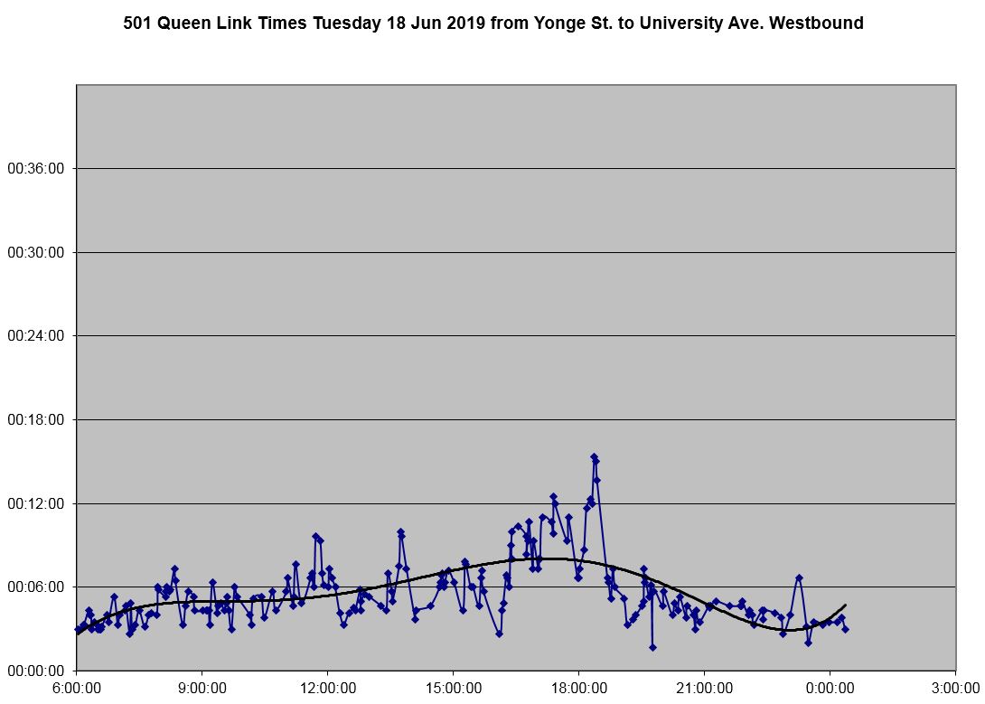
In the heart of the city, right beside City Hall, the longest travel times occur during the PM peak period, with smaller delays at mid-day.

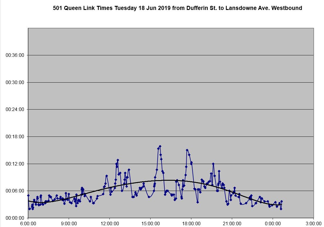
The worst segment in the west end lies between Dufferin and Lansdowne thanks to the junction with Jameson Avenue which feeds into the Gardiner Expressway. Note that there is both a mid-day rise in travel times as well as the shoulder peak effect mentioned earlier.

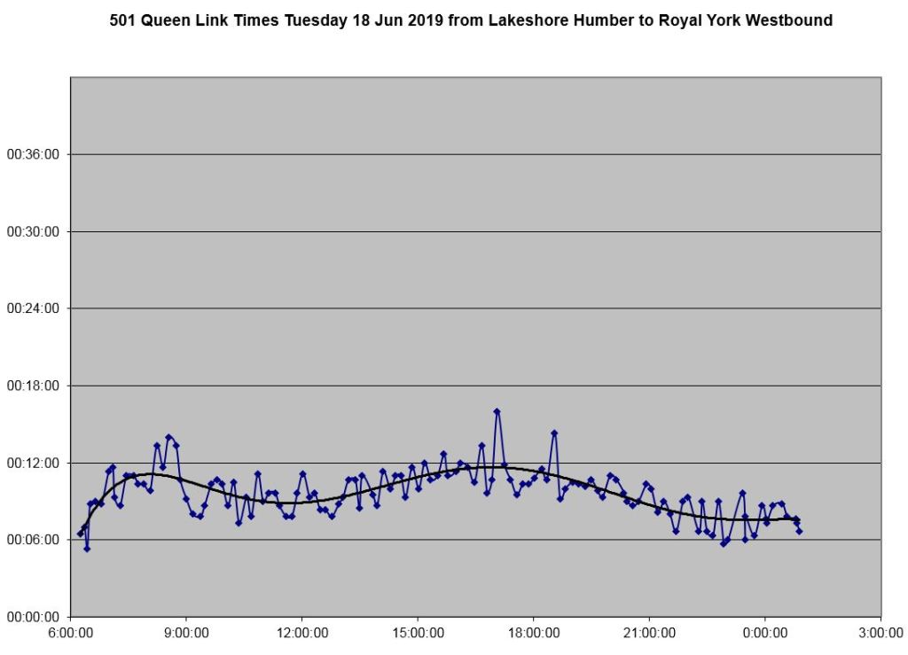
Finally, west of Humber, there is little congestion affecting westbound trips, and this lies mainly in the area west of Humber Loop.

For eastbound travel, some of the same effects occur as westbound, but not necessarily at the same time of day. West of Humber, travel times rise in the AM peak as one would expect for the primary traffic direction.

Similarly, congestion approaching Lansdowne/Jameson builds west of the intersection in the AM peak.

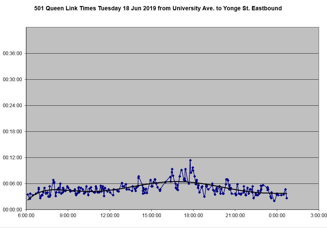
From University to Yonge, there is some congestion in the PM peak, but not as much as for westbound travel. The modest rise in travel time shown here is quite different to the period of TIFF in September when much traffic, including streetcars, diverts off of King Street to Queen. I will use this as an example later in the article.

The full set of travel time charts for June 18, 2019 are below.

Monthly Headway and Link Time Charts

The level of detail in the daily charts above can initially be fascinating especially when researching operations on a day with a known major traffic or weather event, diversion or breakdown. However, each of the charts only shows one day’s data, and one quickly has “information overload” trying to look at many days and circumstances. To get the larger picture of how service behaves, we have to step back and consolidate the data at a weekly and monthly level.

As with the daily charts, the format of the monthly charts is the same for headways and for links. However, for links I also regularly generate charts for multiple segments such as Humber to Yonge on Queen to track patterns over longer distances. If something sticks out in this broader view of the data, one can always drill down to find the source of problems.

Monthly Headway Charts

When I began to build this collection of charts, the first one I produced was a scatter diagram of all headways at a point. My hope was to see most points in a fairly narrow band around the scheduled value with some outliers. However, that was not what actually appeared.

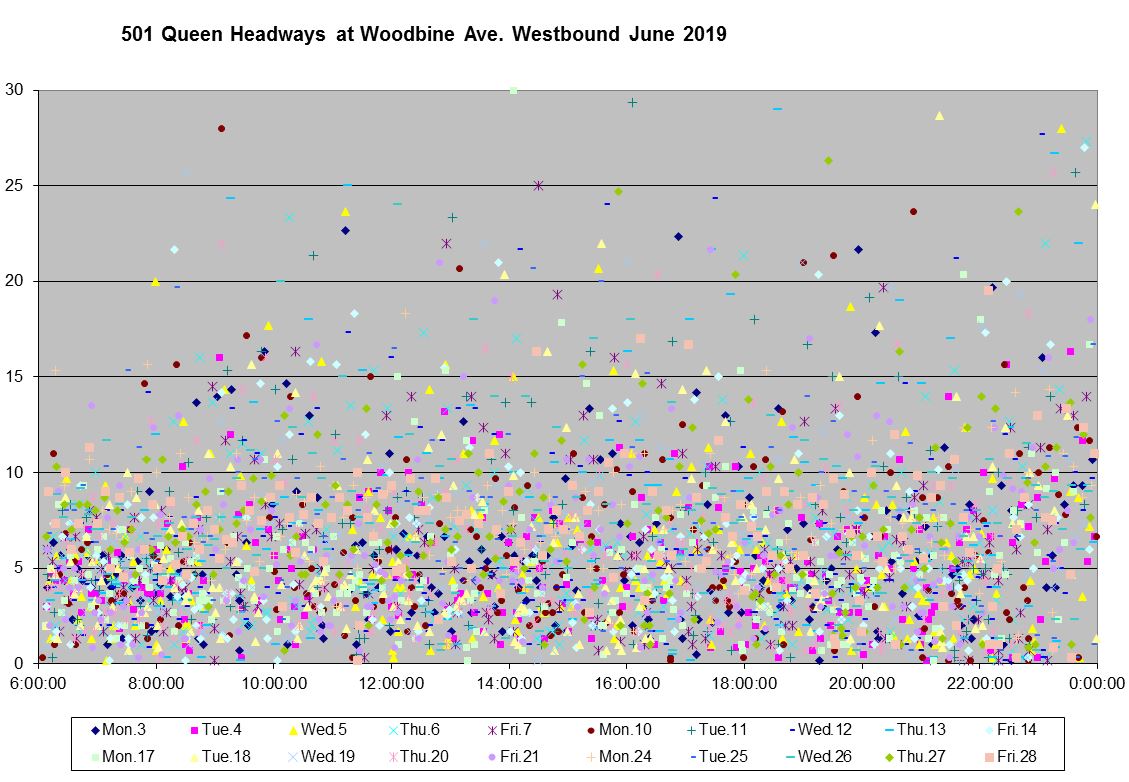
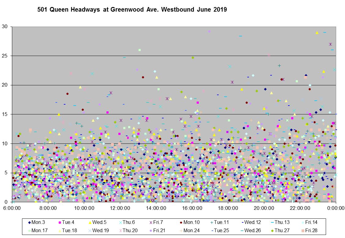
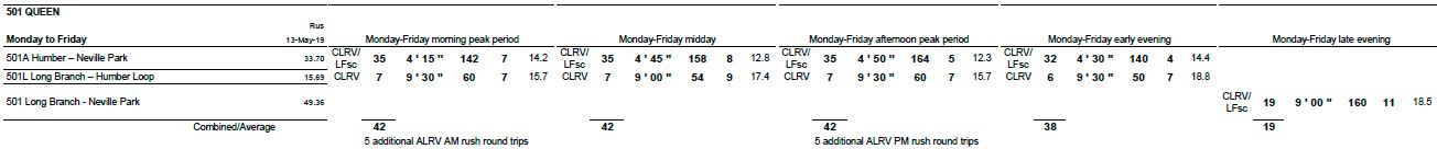
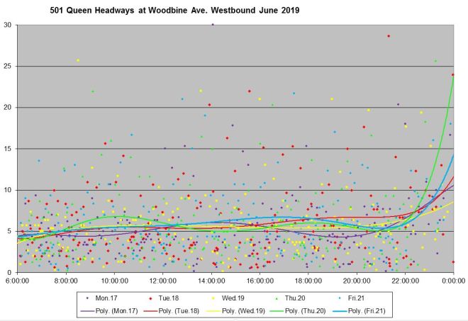
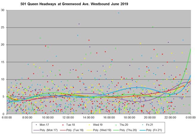
The chart below shows all trips westbound on Queen at two locations: Woodbine and Greenwood in June 2019. Time of day runs left to right, and the headway value bottom to top. Even without any formal statistical analysis, it is clear that most headways are smeared over a band from zero to ten minutes, and higher values are not uncommon.

The situation is worse westbound at Woodbine where short turns at Greenwood Loop and Russell Carhouse strip some trips out of the total.

The scatter diagrams should be a wake-up call to anyone who cares about transit, but we need to dig deeper to see what is going on. A simple calculation is to look at the average headway.

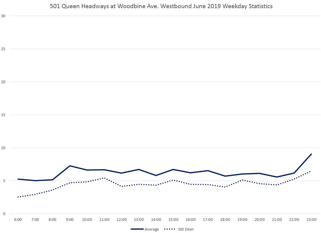
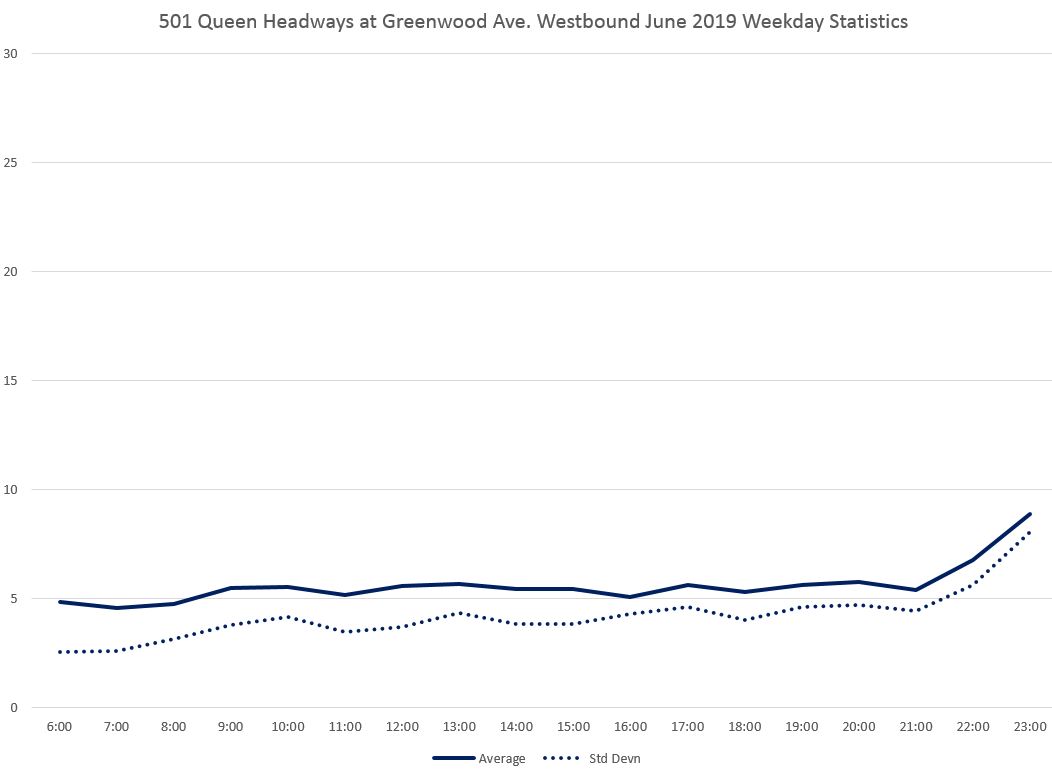
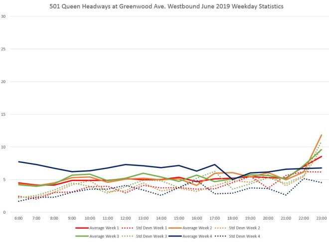
The solid line below is the average value of headways on an hour-by-hour basis for all weekdays. The problem with an average, however, is that it completely masks the actual scatter of values shown in the charts above.

The dotted line shows the “standard deviation” of values and is a measure of how tightly clustered values are around the average. The lower the SD, the smaller the range of values in the overall collection. Roughly two thirds of the headways will lie within one standard deviation either side of the average.

In the chart below, the average lies at about 5 minutes. With the SD value of 4 minutes, this means that about two thirds of headways will fall between 1 and 9 minutes (5 ± 4 minutes). That is similar to the main band in the “cloud” of data points above.

As a technical note, the headway data here are as close to a 100% “sample” as one is likely to get. This is not a survey where a small set of data is used to project values for an entire population.

At Woodbine, the average is higher than at Greenwood for much of the day because of trips that never reach Neville Loop thanks to short turns. The SD value is also higher and close to the average.

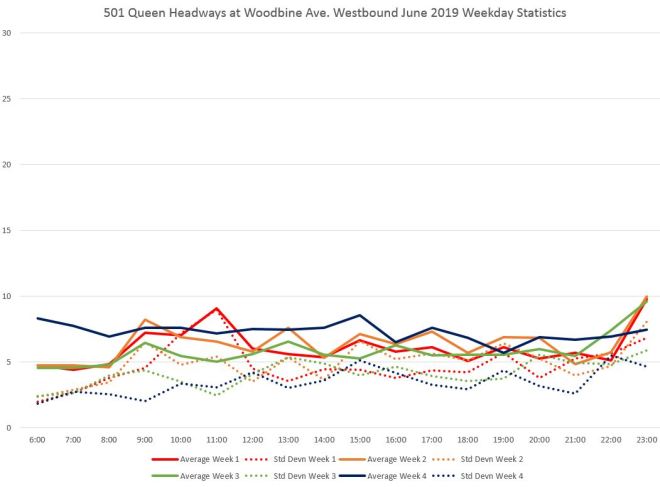
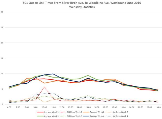
Month-long averages could hide changes within the month, and this shows up when we break down the analysis by week. In the charts below, each week has its own average and SD plot, and we immediately see that the average headway for week 4 is higher than for other weeks. It happens that this marked the transition of scheduled service for CLRVs to the larger Flexity cars with a widening of scheduled headways.

Although the average headway in week 4 is longer, the SD value is only slightly lower than in other weeks. What this means is that the band of data points has shifted upward, but the central portion with most of the points is almost as wide as before.

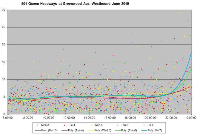
Here are the scheduled weekday headways for 501 Queen for weeks 1-3 of June, 2019, and for week 4 showing the changes (click to expand).

The scatter diagrams can be broken down by week and day to give a better sense of how the headways behave. Week 1 saw much worse service at Woodbine than at Greenwood based on both the average and SD values (red in the charts above).

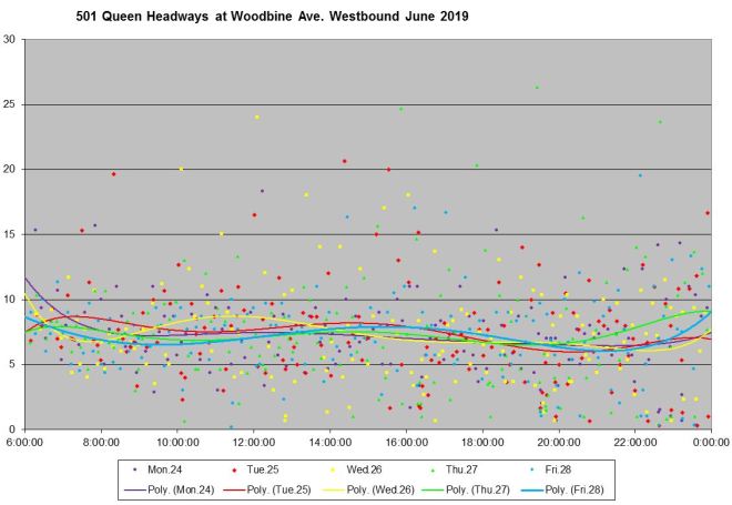
In the charts below, each day of the week has its own colour for the data points and for an associated trend line that threads through the data showing the overall shape. The trend lines at Woodbine are not as uniform as at Greenwood showing both the greater range of headways east of Woodbine Loop and the day-to-day inconsistencies.

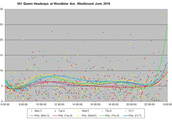
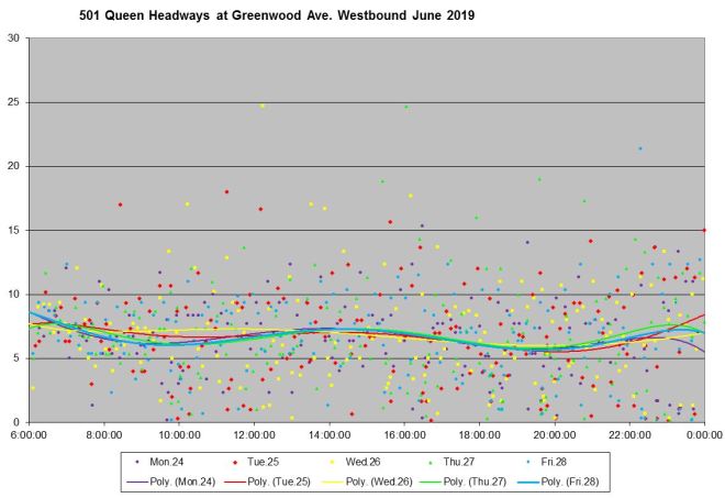
Week 3 does not show as much difference between the two locations, although the service is still far from ideal.

In week 4, the scheduled headways are wider, but the general pattern is similar.

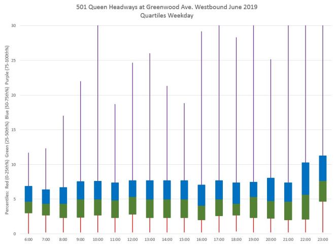
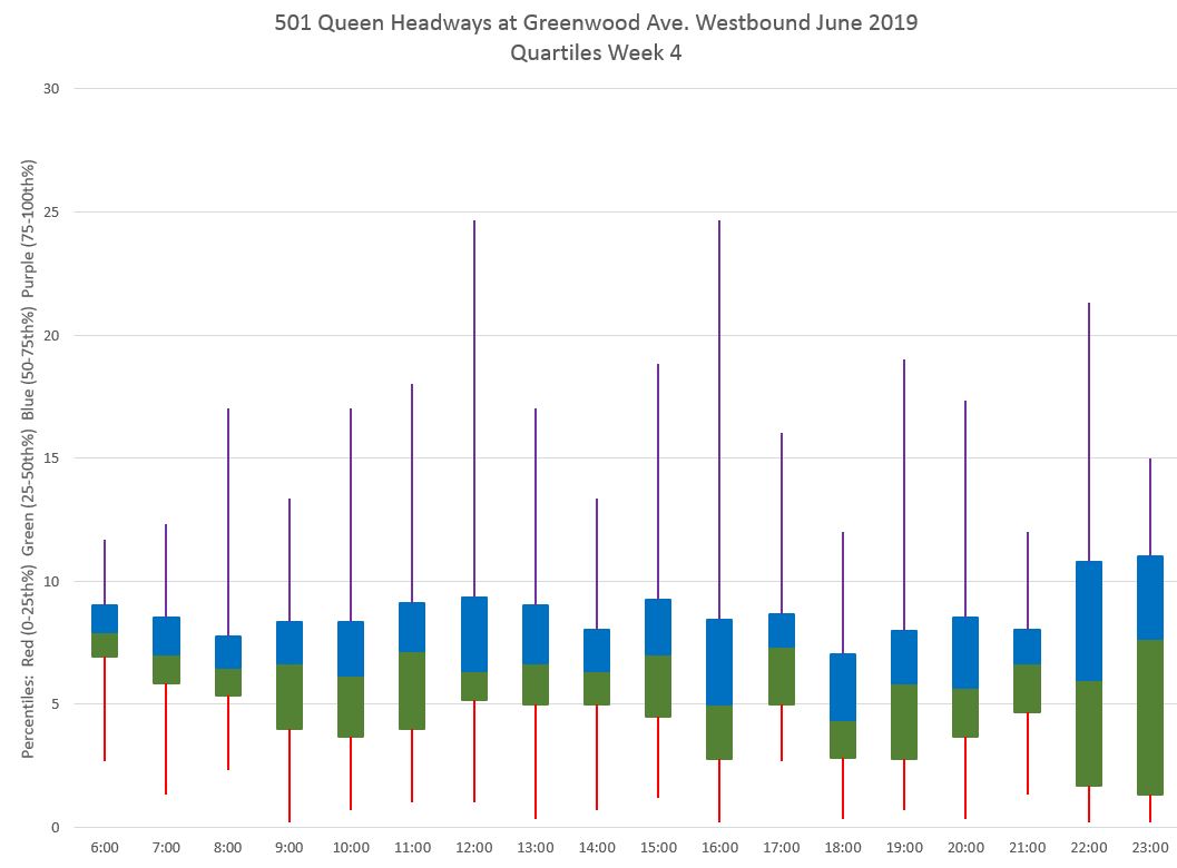
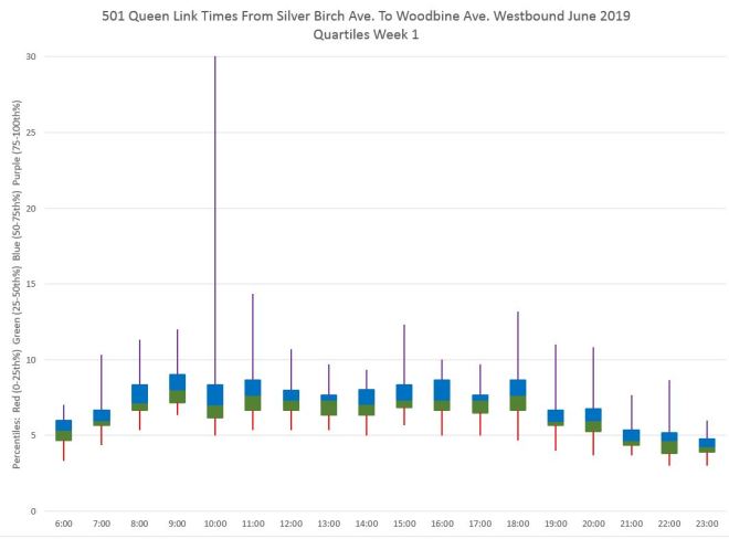
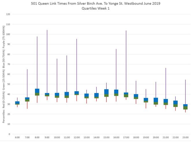
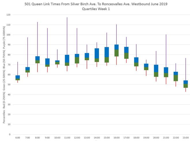
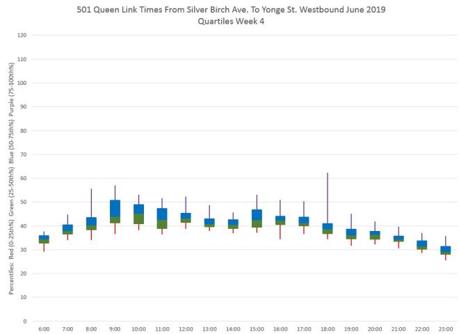
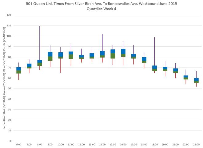
Another way to gauge the range of headways is to break them into quartiles. The charts below are in “box and whisker” format where the middle two quartiles (percentile ranges from 25-50% and from 50-75%) are shown as boxes (green and blue respectively), while the outlying quartiles are whiskers. Ideally, we would like the whiskers to be short, but in most cases here they are not showing that a considerable number of data points lie outside of the central 50% embraced by the boxes.

Note that these charts are clipped at 30 minutes although there are values beyond that level in the data.

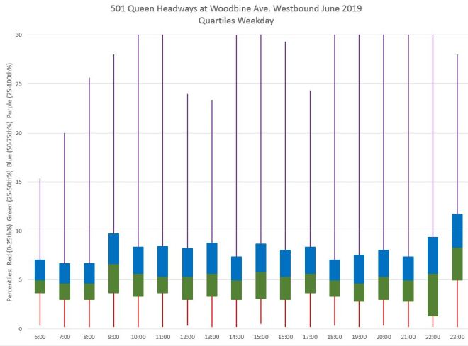
As before, there are problems with consolidation of the data on two counts. There is the schedule change in week 4 mentioned earlier, but also week 1 was particularly bad for short turns as the earlier charts show.

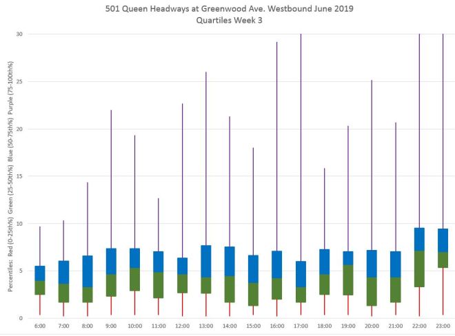
Here is week 3 showing the service before the schedule change.

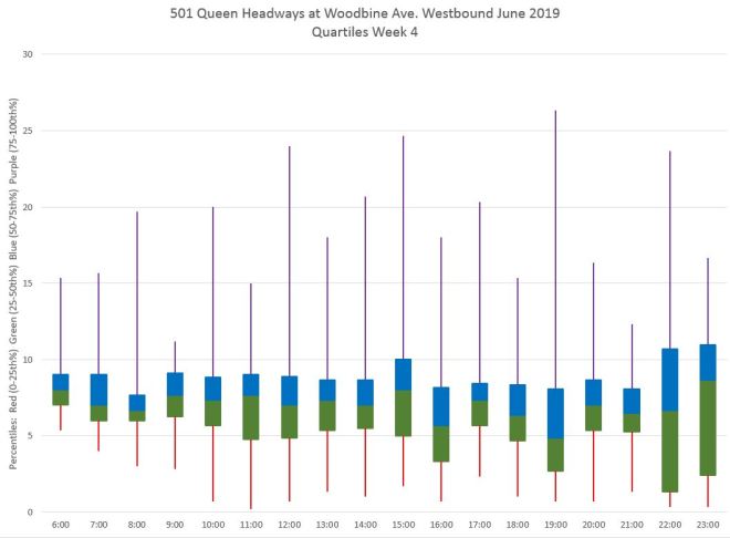
Week 4 shows the service after the schedule change.

The files below contain all of the monthly headway charts above including plots of weekend data not shown here.

Monthly Link Times

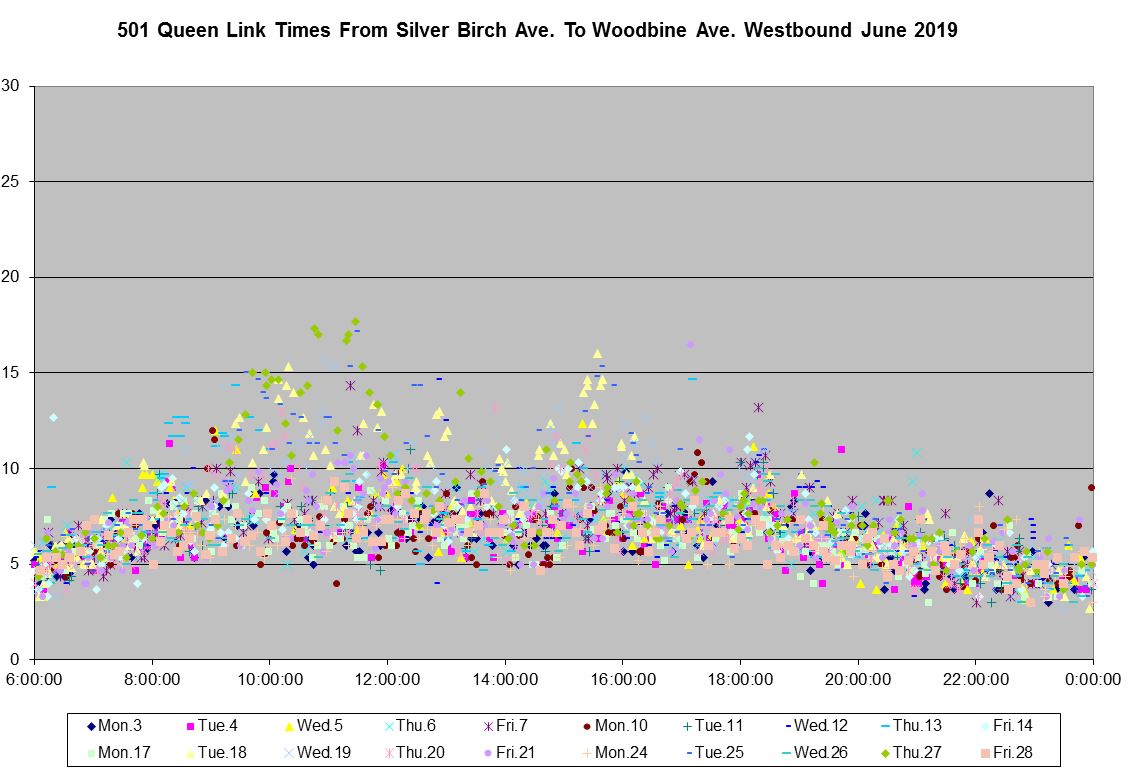
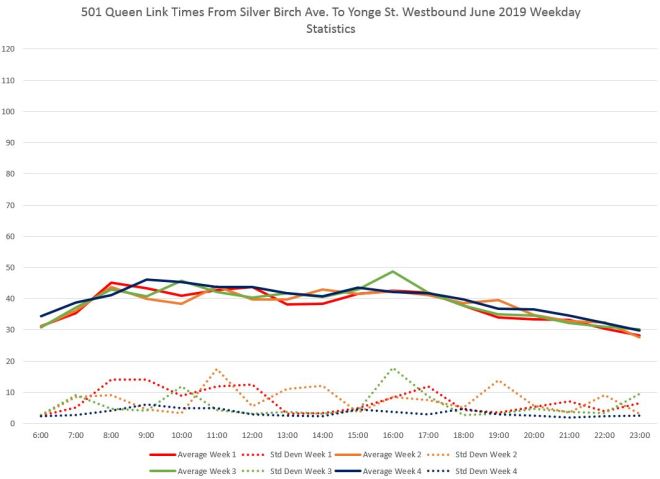
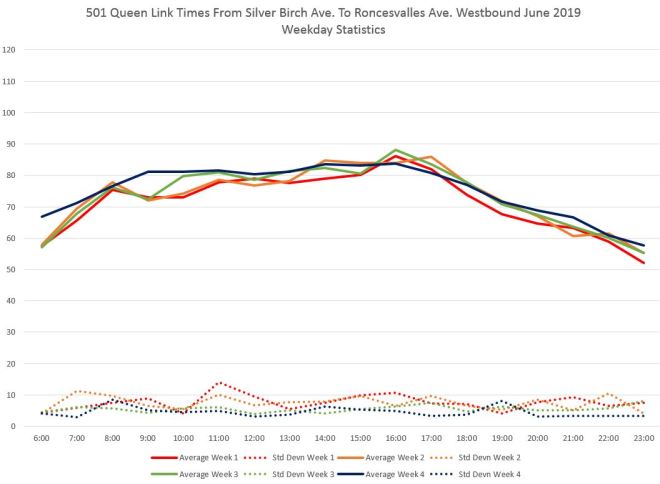
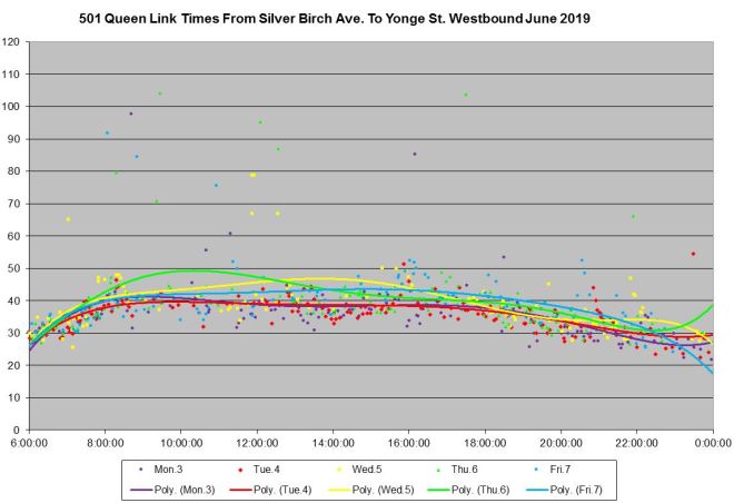
Travel times between points on a route tend to be a lot more stable than headways, although they will rise and fall depending on congestion, stop service time and special events. For June 2019, here are some examples for the following segments of the Queen car.

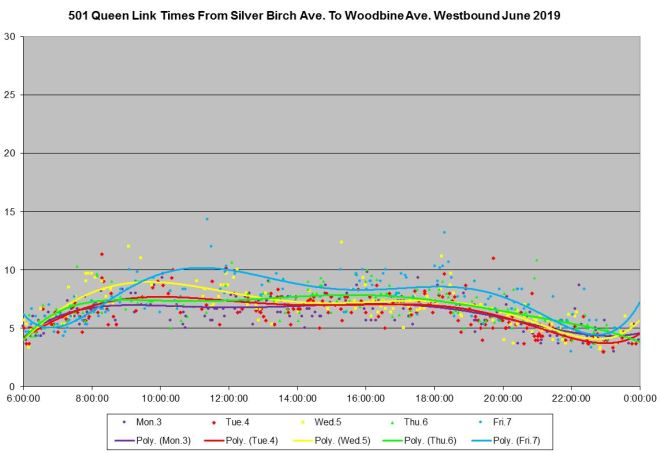
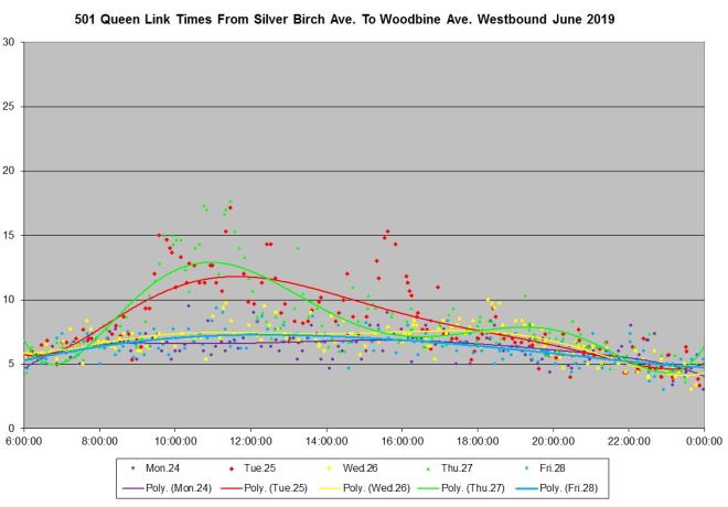
• Silver Birch to Woodbine (note that the scale on these charts is different from those for locations further west)
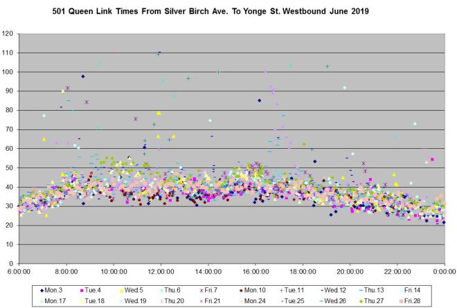
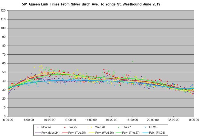
• Silver Birch to Yonge
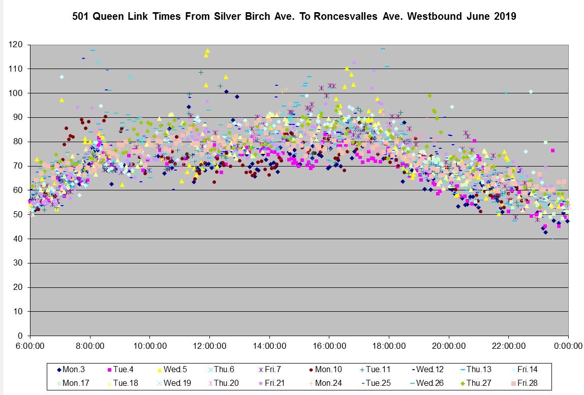
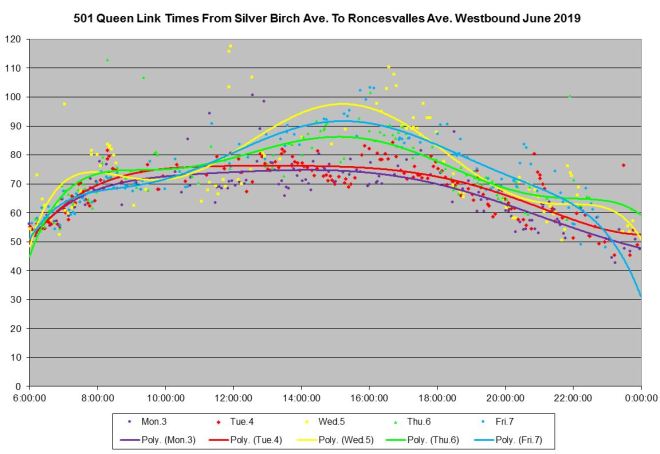
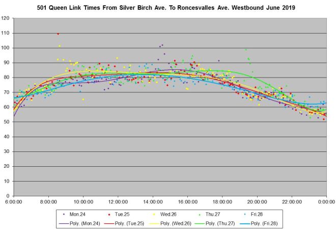
• Silver Birch to Roncesvalles

The full collection of data points shows that even through The Beach to Woodbine there is a band about 5 minutes wide which is rather large considering that the average lies near 8 minutes. Between the peaks, this can get worse. The light yellow triangles are data for June 18 for which a detailed service chart is linked earlier in the article, and which shows that the congestion built up westbound to Woodbine. The green diamonds are for June 27 when a similar problem developed after the AM peak until after noon. This is an example of how conditions are not always the same on a route from day to day.

For the data between Silver Birch and Yonge, there are a scattering of points well beyond the main band of the data. Examination of the daily service charts shows that these cars laid over for an extended period at Russell Carhouse, probably because no operator was available for a crew change, and then continued on their way.

There is also a collection of points after 4 pm on Friday, June 21 with very long travel times. This was not one of the better days for the Queen car. A delay westbound at Greenwood (for which no eAlert was issued) held seven cars over a period of half an hour. When these cars reached Boulton (east of Broadview), they were held for another 40 minutes for what the eAlert described as a “mechanical problem”. This created a one hour gap in service into which only one car was short turned and that only as the delay was finally clearing. June 21, 2019, is a day worth examination in detail, but that is beyond the scope of this article.

Finally, for trips across the city from Silver Birch to Roncesvalles, the band of data points is about 20 minutes wide showing how much conditions can vary from trip to trip and day to day. The band is slightly wider in the PM peak periods, but there are clearly still problems throughout the day. This is important for discussions of transit priority because changes that only address peak conditions would leave much of the service (and by extension many riders) with no improvement.

The charts in this section are intended to illustrate how important details can be lost by to great a level of consolidation, and how the challenge is to find an intermediate point of balance between a summary view and too much detail.

The same data presented as averages and standard deviations tell the same story in a mathematically more formal manner. However, they hide a lot of detail, notably the effect of isolated events that, within a collection of 20 days’ data, don’t move the lines very much.

Some of this detail is restored if the data are presented on a daily basis, collected into weeks. The charts below show data for week 1, June 3 to 7, both with trend lines and in box-and-whisker format.

The following set show the data for week 4 which is much different.

The full chart sets for the three segments are linked below.

Travel Time Histories

The data underlying the monthly link charts in the previous section can be consolidated to provide a view of changes over a longer period. I created this type of chart for analysis of the King Street Transit Priority Project in order to display the “before and after” conditions through the pilot area (Jarvis to Bathurst) and for comparison with other parts of the route.

The same chart structure can be used to look at headway histories, but I will not include any here as they are the same format.

Assuming one has the source data, one can track over a very long time to determine whether there are any long-term patterns such as gradual growth of congestion pushing travel times up and/or reliability down.

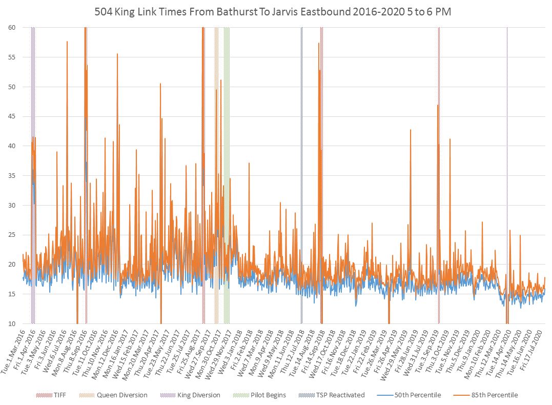
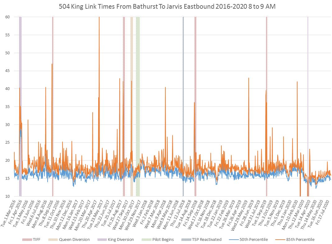
The chart below shows travel times on weekdays from March 2016 to July 2020 on King between Bathurst and Jarvis. In this case rather than showing the quartiles, the chart tracks the 50th percentile (median) and the 85th percentile. Two major changes in the character of the data are visible:

• At the beginning of the pilot, November 2017, there is a slight reduction in the values but a big decrease in the day-to-day swings in effect “clipping” off the tops of very large spikes in the pre-pilot era (except during events that undid the benefits such as TIFF).
• There is a drop in March 2020 corresponding to the traffic reductions due to the covid pandemic.

The chart for the 8-9 AM peak hour is different in that it shows little change when the transit priority pilot began, but it does mark a drop post-pandemic, although this is slowly rising in the most recent data. (I will examine the 2020 data for King and other routes in detail in a separate article.)

Travel Time Comparisons

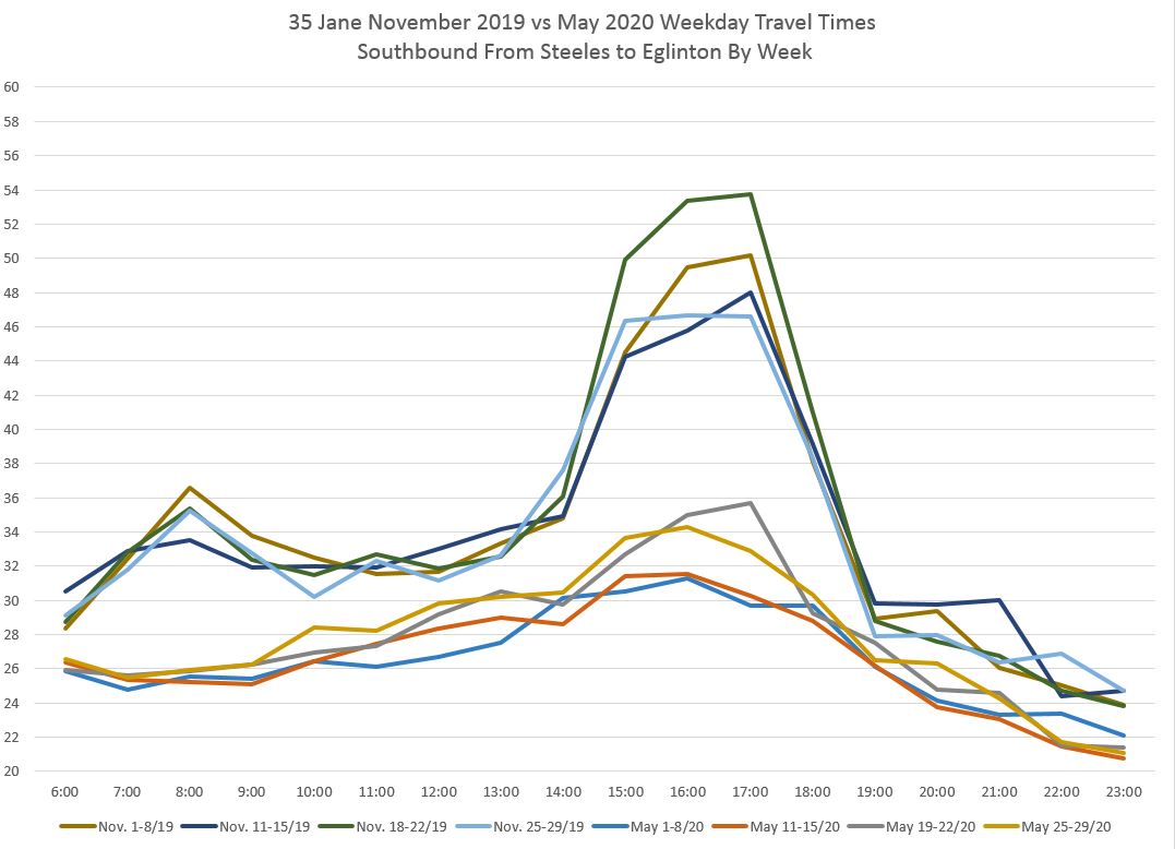
The travel time data can also be grouped by week or month to track the evolution of values. The chart below was created for a review of the effect of covid-19 on traffic congestion on the Jane corridor. These are the same weekly averages that appear in the monthly charts, but consolidated for comparison.

Depending on how clearly there is a distinction between two groups of data, a chart with too many lines can simply become confusing rather than illuminating. This chart includes values for selected weeks for all times of the day, whereas the history chart for King above tracks all days, but for a specific time period.

Speed Comparisons

The travel time charts shown above tell us how long it takes to get from “A” to “B”, but they do not show us how vehicles spend their time in between, nor how this varies during the day.

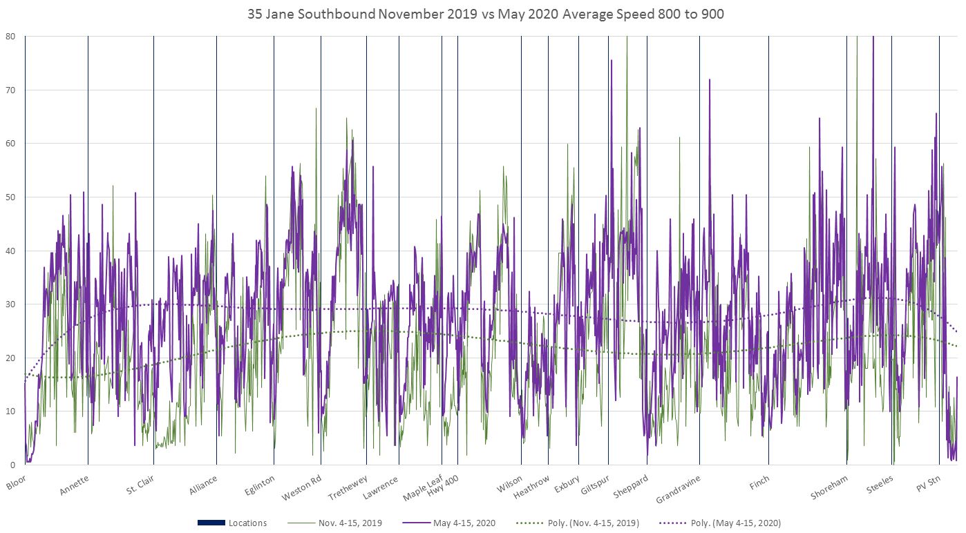
Because all vehicles are tracked by GPS with reports of their location every 20 seconds or better, it is possible to know moment-to-moment how fast they are travelling. When the values are combined, we get a profile of the operating speed along a route. The chart below compares the average speed of buses on 35 Jane by location during two periods before and after the drop in traffic level in 2020.

The data are for southbound service with Pioneer Village Station at the right and Bloor Street at the left. There is a characteristic sawtooth shape to these charts where each dip corresponds to a stopping location. If buses operate slowly only to stop, then the dip is narrow. However, if there is congestion in advance of the stop caused by intersection capacity, then buses will slow before they reach the stop, and the dip will be wider.

The height of the peaks corresponds to the period when buses are running at speed. The length of time they can do this depends on both traffic conditions and stop spacing. If stops are far apart and there is little congestion, then buses will sustain a higher speed for longer.

In this chart, the pre-covid data from early November 2019 (green) are compared with the data from early May 2020 (purple). The dotted lines are trend lines calculated by Excel as a best fit to the overall shape of each set of data showing the degree to which the values differ along various parts of the route.

Each chart covers one hour’s operation, but shows the entire route.

Here is the morning peak hour from 8 to 9 AM.

Here is the afternoon peak from 5 to 6 PM showing how much different conditions apply in the PM peak.

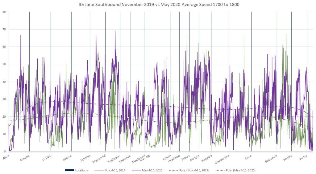
A full set of these charts is available in the Jane corridor analysis article. Within the full set of hourly charts, one can step from hour to hour to see how the speeds and delays along the route evolve. There are locations where operations were definitely slower in fall 2019, but other where this is not the case. Jane is a route with substantial differences in speeds, but not all routes show the same effect and even Jane varies by location and time-of-day. This feeds into discussions of transit priority schemes by showing where and when there actually are problems that might be addressed.

Although the charts here compare the same route under two different traffic conditions, I have also used this for comparisons of transit modes where, for example, buses replace streetcars.

A caveat: the charts only show the speed between stops, not the time taken at each stop to serve passengers and/or to wait for traffic signals to clear. I have yet to concoct a chart that displays this clearly as it is difficult to know why a vehicle is stopped, only that it is not moving. For a location with a farside stop, signal delay can be separated from stop service time, but most stops are nearside and the two delays combine into one.

Service Capacity Charts

The capacity of service actually operated is rarely equal to that scheduled for a variety of reasons:

• Vehicles do not arrive in the expected quantity within a time period. For example, during a peak hour where 15 are expected (one every 4 minutes on average), one might see fewer or more vehicles. This is especially true if the location in question is served by multiple routes any one of which might be disrupted. Another common way vehicles can be missing is if they are scheduled as trippers that may or may not operate depending on operator and vehicle availability.
• Vehicles actually operated do not match what is scheduled. The most common example of this is the arrival of a standard sized bus where an articulated bus 50% larger was scheduled, or a standard length streetcar (CLRV) in place of an articulated one (ALRV) or a new Flexity. On the streetcar system, there is now only one vehicle type and so this particular problem has disappeared.

Calculating the actual capacity provided at a point is easily done simply by counting how many vehicles pass within a given timeframe. This information is already available in the daily headway files described earlier in the article, and a program simply collates all of the data for the location and period of interest. The raw vehicles counts multipled by their capacity (as defined in the service standards) gives the actually provided capacity.

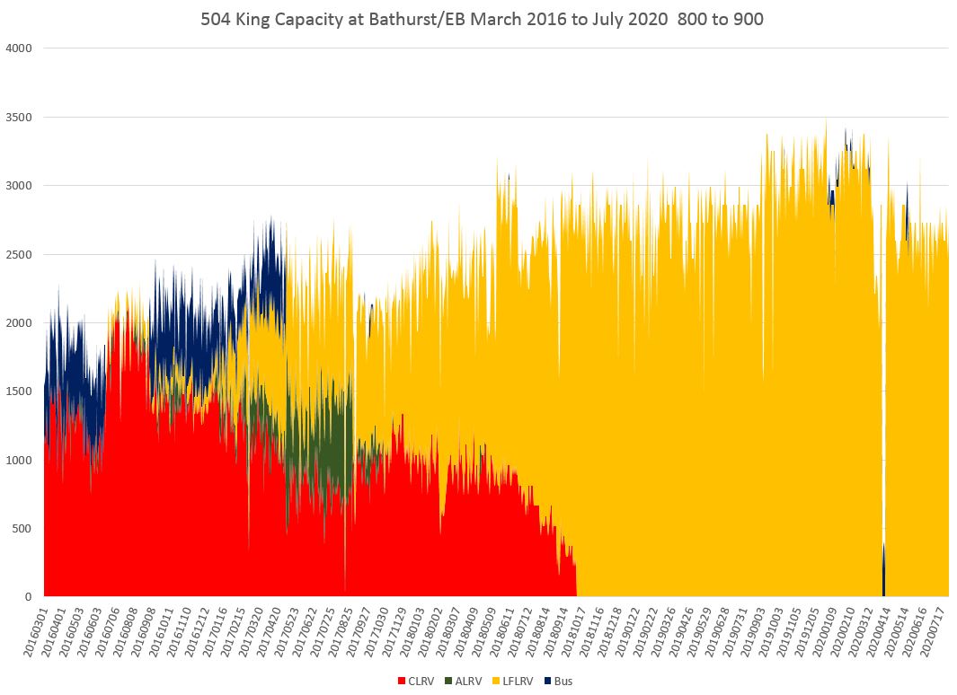
The following chart shows service on King Street eastbound at Bathurst Street between 8 and 9 AM from March 2016 to July 2020. Note that the capacity of vehicles after March 2020 has not been adjusted to compensate for covid loading standards, but reflects pre-covid values.

The chart is colour coded to show the contribution of each vehicle type to the total. (The notch in April 2020 corresponds to a period when streetcars diverted to Queen Street due to track repairs at Shaw Street. A limited bus shuttle filled the gap.)

An important point about this chart is that it shows the large variation in capacity as actually provided. If service ran at the scheduled frequency and “on time”, there should be no variation in the value from day-to-day. In fact from mid 2018 to mid 2019 there is a regular variation in a range between 2,500 and 3,000 with occasional dips below 2,000.

Service was improved in fall 2019 and the peaks reached into the 3,300 range, but there has been a post-covid cutback to about 2,700. Of course the practical capacity when allowing for distancing is considerably lower.

TTC Service Quality Metrics

The time has come to talk about how the TTC measures service quality. Their analysis is based on “on time” statistics, where that phrase is defined as not more than one minute early and not more than five minutes late. This is a not uncommon approach, but it does not tell us much about the service riders actually get.

There are three big problems with this metric.

First, it is calculated only at terminals, not at intermediate points. This tends to show service in the best possible light when vehicle spacing is fairly regular. As shown earlier, that condition does not last long, and gaps/bunches form along a route.

Second, a six-minute window might make sense on a 30 minute headway where one definitely does not want a bus to be earlier than expected, but not outrageously late either. For a service operating every 10 minutes or less, a six-minute leeway in being “on time” allows bunching to be considered as acceptable.

For example, if buses are scheduled at

8:00, 8:10, 8:20, 8:30, 8:40, 8:50, 9:00

they could actually run at

8:05, 8:09, 8:25, 8:29, 8:45, 8:49, 9:05

and all be counted as “on time”. Riders would routinely encounter 16 minute gaps followed by two closely spaced buses. If the scheduled service were even more frequent, then two or even three vehicles could run nose-to-tail and be “on time” for the purposes of TTC management statistics.

Third, the TTC only reports averages and usually does this over extended periods that mask the effect of weekly, daily and hourly variations.

Riders do not care about “on time” for frequent services, they want vehicles to show up at regular intervals with moderate loads. Riders do not ride average services, they ride what actually shows up as and when a car or bus deigns to arrive.

TTC management’s attitude is that if service is “on time” at terminals, then the rest of the line will take care of itself. This is utter nonsense.

Service does not leave terminals well-spaced, and the headways become more erratic as vehicles travel along their route.

The fact that bunching can cause typical headways to be much longer than scheduled causes service to be equivalent to one with many short turns even though on paper there are none. Two vehicles every 20 minutes is not the same as the same vehicles 10 minutes apart.

The TTC briefly published On Time Departure Reports for each route, but this lasted only from April to August 2018, and nothing has replaced them.