
Updated October 11, 2018
An updated set of charts has been added which show the evolution of headway values across the route by time of day, including an improved version of the “box and whisker” chart format. Scroll down to the end for this update.
Updated October 9, 2018
A substantial section has been added to this article with replies to many of the issues received in the comments and examples of revised and additional charts. Thanks to all who have commented on this.
Errata
I noticed that the data for the period from 6-7 am on 505 Dundas at Broadview Station has an unusually high value for headways below two minutes. On investigation I discovered that this was caused by garage trips that were inadvertently included in regular service. This only happens for buses that arrive via Danforth rather than via Broadview because of the geometry of the screenline in my model at Broadview/Danforth. This caused these trips to be counted twice: once on the way into service, and again when they left Broadview Station. Charts in the original article that were affected by this problem have been replaced.
Original Article
An ongoing issue for transit riders is the question of service regularity. TTC Service Standards call for vehicles to leave terminals no more than one minute early and no more than five minutes late. That by itself provides a huge amount of variation within “acceptable” service, but there is no attempt to measure route behaviour once vehicles leave the terminals.
One unfortunate effect of Andy Byford’s term at the TTC was the creation of service metrics without necessarily making things better for riders.
Riders do not care if a bus or streetcar is “on time” on many routes, only that they show up regularly. That is the whole idea of “frequent service” – you don’t need a timetable, you just show up and travel without an excessive, unpredictable wait.
I have been wrestling with how to illustrate the problem for some time. As part of preparation for a series on suburban bus service, I wanted to create a measurement that would be fairly easy to understand and which would allow comparison from route to route and place to place.
This article presents the work-in-progress for suggestions to improve or add to the charts before I start publishing data for many routes.
Source of Data
As with all analyses published here, the source data are the TTC’s vehicle tracking records from the “CIS” (Communications and Information System) which, among other things, collects the GPS location of vehicles every 20 seconds. The transition to a replacement system “Vision” is underway, but all of the data I have used here comes from routes that were still operating under CIS at the time.
Along the length of routes, I have defined timepoints where the passage of vehicles is used to construct an “as operated” schedule from which headways at the timepoints and travel times between them can be calculated. [Chart updated Oct. 9/18]

From this chart it is quite clear that there is both a wide range in headway values leaving the terminal for 505 Dundas buses on the day shown, and that many buses leave on very short headways with pairs of vehicles travelling close together. The offsetting effect of course is that there are wide gaps between these groups.
A set of charts showing how this pattern evolves along the route is linked below. [Updated Oct. 9/18]
The situation varies from route to route with a common situation showing less spread in headways at the terminal, but quickly a pattern of bunches and gaps evolves as vehicles move along their route.
Consolidating the Data for Charts
The headway data for each timepoint has been summarized for all weekdays in a month by hour of the day and in two minute increments.
The first attempt I made at this used bar charts to show the distribution of headways at a point hour by hour. These are expressed as percentages of all trips, not as raw counts, so that values can be compared between locations and times.
For each hour, the red bar shows the proportion of headways that lie from zero to just under two minutes. Orange shows two to just under four minutes, and so forth through purple which shows trips at or above a 12 minute headway.
It is no surprise that the higher values dominate late at night, but through much of the day the lower values dominate. [Chart updated Oct. 9/18]

It does not take long after buses leave Broadview and Danforth for the headway distribution to shift. The chart below shows values at Dundas Street where the red bars (under two minutes) are the highest for most of the day. This indicates that a good deal of service is operating as closely-spaced pairs (or worse) of buses.

By the time service reaches Yonge, the pattern is even stronger.

Although these charts are colourful, they are also hard to read because separate charts are needed for each location and they are “busy” in that extracting specific information takes some study. This led me to an alternative way to display the data.
Given that the concern for this analysis is bunching (short headways), the data we really want to see is in the red bars (under two minutes). This leads to a chart consolidating the two-minute data for all locations along the route. Because of the number of timepoints in the analysis, this information has been broken into two charts for eastern and western sections of the route.
The pink line in the first chart shows that leaving Broadview Station, vehicles on short headways accounted for 15-20% of trips for much of the day. However, the proportion rises at Broadview/Dundas (red) and even moreso at Parliament (dark red), Jarvis (orange) and Church (light blue) with about one third of all trips on short headways. The values drop at Yonge (green) probably due to the combination of stop service time and the throttling effect of traffic signals, but rise again a short distance to the west at Bay (dark blue). [Danforth to Bay chart updated Oct. 9/18]

The situation continues on the western portion of the route.

For comparison, the average headways are shown below. Note that daytime values at Lansdowne, Roncesvalles and Bloor are higher than points further east probably due to short turning of buses to compensate for the construction at Lansdowne and the diversion via Dufferin and College. [Danforth to Bay chart updated Oct. 9/18]


Another way to look at headway reliability is the standard deviation of headway values. This value indicates the degree of spread in values, and the smaller the number, the more tightly clustered around the average (mean) the values are. Commonly, two thirds of values lie within one SD either way from the average.
Except for early in the day, the SD values lie in the area of five minutes, and this is consistent across the route. These values indicate that headways span roughly ten minutes for a substantial portion of trips, with an even wider range for all trips.
The spike in values at Spadina was caused by a single data point where a two-hour blockage and diversion meant that no vehicles crossed the screenline at Spadina for an extended period. The change in the SD value is much less than 120 minutes, but that one very large value can have an effect. Normally such data points would be filtered out, but I have left that one in to show the effect. [Danforth to Bay chart updated Oct. 9/18]


Looking at Another Route: 52 Lawrence West
By comparison, here are similar charts for the 52 Lawrence bus. This route is different from 505 Dundas in that all service does not operate over the entire route. As of April 2018, some buses only came as far east as Lawrence West Station, and at the western end service is split between the Airport and Westway branches.

West of Lawrence West Station, headways under two minutes dominate the chart for much of the day, and the situation becomes more pronounced by Keele Street where the 0-2 and 2-4 minute bars are the overwhelming majority.


Looking at data along the route, the two-minute values are lowest at the airport because scheduled headways here are so wide that bunching should be quite rare. That said, it is clear that some bunching does occur during the PM peak and early evening.
Leaving Yonge Street, the proportion of bunched service varies through the day with the worst values at the ends of the two peak periods. As on Dundas, the proportions grow as bunching becomes more severe along the route hitting a high point at Scarlett Road. This very high value probably reflects an operating practice where buses on the two branches make no attempt to maintain even headways near the point where the route splits. A related problem is the degree to which inbound service merges well (or not).
The values fall back at Martin Grove and Dixon because there is less scheduled service and therefore less opportunity for bunching. Even so, the degree of bunching here is not trivial ranging above 20% for most of the day.

Average headways show the service design along the route with the shortest scheduled headways between Lawrence West Station and Scarlett Road, another band for locations east of Lawrence West, still higher at Martin Grove, and higher still at the airport.

Standard deviation values on Lawrence are consistent for most locations, although they are noticeably higher on Dixon Road and at the airport.

The complete sets of charts for 52 Lawrence are linked here. Charts for 505 Dundas are at the end of the article following the updates.
Request for Comments
Please let me know what works and doesn’t work for you as a reader in looking at these charts, what might be done to improve them, and how these data can best be displayed for easy understanding.
Updated October 9, 2018
Many comments came in with suggestions on changes in the way that the headway data might be displayed to give a good sense of service quality. Because there is some overlap in the suggestions, and because it is preferable to include new illustrations in the main article, I have consolidated responses here rather than in the individual comments.
I have only included updated samples here for 505 Dundas as this gives the general feeling of what works and what does not.
Headway vs Waiting Time
Many people noted that riders experience waits, not headways, and that some way of translating what riders see into an index of some kind is needed. Alternatively, some explicit measurement of how long one is likely to have to wait at a given time of day and location.
This inevitably runs into the common analysis problem of averages versus a level of granularity that reveals something useful. For example, a route might have an average headway all day of five minutes, and hence an average wait time of 2.5 minutes. However, if buses come every 5-5-5-5-5-5 minutes the experience is quite different from that of 1-9-1-9-1-9. Both of these are half an hour’s service, but most riders will see two closely spaced buses and will have an average wait time of 4.5 minutes (half of the 9 minute gap). For vehicles running truly in pairs, 10-0-10-0-10-0, the average wait is 5 minutes.
Suppose this is a stop that serves 1 rider per minute, or 30 per half hour. With buses exactly the same time apart, all 30 of these riders will have a 2.5 minute average wait time for a total of 75 wait-minutes. In the second example, 3 riders will wait .5 minutes each (1.5 wait-minutes) while the other 27 will wait 4.5 minutes each (121.5 wait-minutes) for a total of 123 wait-minutes.In a situation where vehicles travel in pairs, 30 riders wait 5 minutes each for a total of 150 wait-minutes, or double what would be the case with the advertised service. Actual service on any route will lie somewhere in between and will vary from day to day.
There are caveats about this, of course, notably that some riders will wait for the second, presumably less-crowded, vehicle while others will pile onto the first thing that shows up. The riding experience will be a combination of a longer-than-expected wait plus crowding that could very well exceed the TTC’s Service Standards.
Those standards are based on averages and make no allowance for unevenness in crowding between buses. There is a compensating factor in that the service design load is lower than the crush load on the assumption that room must be left over for surges, most typically caused by uneven headways. This brings up major problems when politicians looking for “efficiency” say “but you can fit more people on the bus”. Yes, of course you can, but in the process more buses will be full and will turn away riders. Conversely, the cheapest way to create capacity is to run properly spaced service because there is a better chance that all of the space provided on vehicles will actually be used. Even on an overloaded route like the subway, it is no secret that regularly spaced service provides a better experience, relatively speaking, than situations where there is even a minor gap.
The TTC does not regularly publish vehicle loading counts, and on the occasions this does happen, data are averaged over periods such as the AM peak rather than being broken out within hours or percentiles to show the degree of variation a rider will experience. Moreover, loading counts hide would-be riders who simply could not get on vehicles, or who had a multi-vehicle wait to board.
One goal of my analysis is to reveal the degree to which actual operations differ from ideal, let alone the rather generous “standards” by which the TTC measures service quality. The TTC measurement is based on “on time performance” relative to schedules. This is an utterly bogus index for frequent service because the schedule is meaningless to riders. They just show up at a stop and expect a bus or streetcar to appear. That’s what “frequent service” means, and riders want regular spacing. If it is on time so much the better, but a six-minute “on time” window around the schedule allows “frequent” routes to run in bunches while hitting all of the management targets. The problem is compounded, as shown in the data already published here, because even a tolerably spaced service at the terminals (where the TTC measures reliability) quickly degrades into pairs (or worse) of vehicles only a few kilometres down the road.
Because bunching puts the lie to claims of good service, I concentrated on the proportion of service that operates on headways below two minutes. If this proportion is high (and sometimes it reaches 40%), then there will be corresponding set of much wider headways between these bunches of vehicles.
As for including a target value in the charts, this would only apply where all ranges of headways are shown, not just the below-2-minutes group. One challenge with this is that the scheduled headway is not the same at every time and location on a route. for example, in the transition between periods, a “wave” of midday headway works its way across a route from the terminal (or from wherever vehicles go out of service). The target headway may not be the same at 9 am as at 9:30 or at 10:00, and comparing actual headways to one value could be misleading. However, a comparison to the actual average headway could allow calculation of ranges either side of the average, whatever it happens to be. I will return to this in a future update.
A General Note About Percentages, Counts, Averages and Standard Deviations
The charts I have produced are based on percentage values, that is to say what proportion of the service operated within a specific range of headways. If raw counts of vehicles are used, the variation in counts from hour to hour and location to location brings on its own problems, notably that direct comparison between time periods, locations and routes is not possible because the number of vehicles for any one grouping varies. Conversely a statement such as “thirty percent of trips are at a two minute headway or less” is a consistent measure, and the sort of thing that could be converted into a service standard (e.g. a target upper bound on short headways).
Averages hide a lot, and this is the problem with much service quality reporting. Looking only at average headways, while ignoring actual headway patterns, masks the effect that most would-be riders see the gaps as they wait, and wait, for a vehicle to appear. Moreover, the relative crowding of vehicles (or even pass-ups on busy sections of a route) caused by gaps and bunches goes unreported. The “average rider” sees a bus that shows up less frequently than advertised and is overcrowded when it arrives. A closely-following bus can take on the load, but the rider still had the long wait for two or three buses to arrive in a pack.
However, something averages do show us is the changes in vehicles/hour (the inverse of the average headway) along a route. Specifically, if short turns are common, the average headway will rise beyond the point where many vehicles turn back. A combination of a high average headway and a high proportion of short headways is a recipe for disastrously bad service.
As for the Standard Deviations, this is a measure for those with an interest in the dispersion of data values. If the SD is small, then most of the observed headways are close to the average. This should also correspond to periods when the percentage of very short (or long) headways is low. However, as the SD rises, so does the spread in observed headways. On both of the sample routes used here, 505 Dundas and 52 Lawrence, much of the service operates with an SD roughly equal to the average indicating that over half of the vehicles operate at headways from zero to double the advertised value.
The SD is a useful value because it is independent of the actual value of the average. For example an SD of 3 minutes yields a six minute range of commonly observed values regardless of whether the scheduled headway is 5 or 15 minutes.
Some readers asked for a “box and whisker” chart, and I have included a sample below.
Each of these measures will have its adherents, and different measures reveal different things, although clearly some are more technically oriented than others.
Display by Location Rather Than by Time
Several of the charts in the initial article are organized with time along the x-axis and a separate chart line for each location. Many suggested that this arrangement be swapped so that the locations along a route are on the x-axis with a separate chart line for each hour of the day. I agree that this swap improves understanding of how headway reliability evolves and declines over the course of a route, but as others pointed out, this makes for a lot of lines (one per hour) on the chart.
One suggestion was to use line textures to clarify what was what, although this still can leave a very busy chart that takes careful study to understand. As an alternative, I have broken the chart into four time periods: am peak, midday, pm peak and evening. This reveals the way that headway reliability, measured as the proportion of trips at under 2 minutes, evolves quite clearly. The all-day pattern is easy to see by switching back and forth between the four chart pages.
The first chart shows the all day data organized by location east to west and by hour with different dash patterns for each period of the day. This is a messy chart, but things become much more obvious when it is broken apart in following examples.
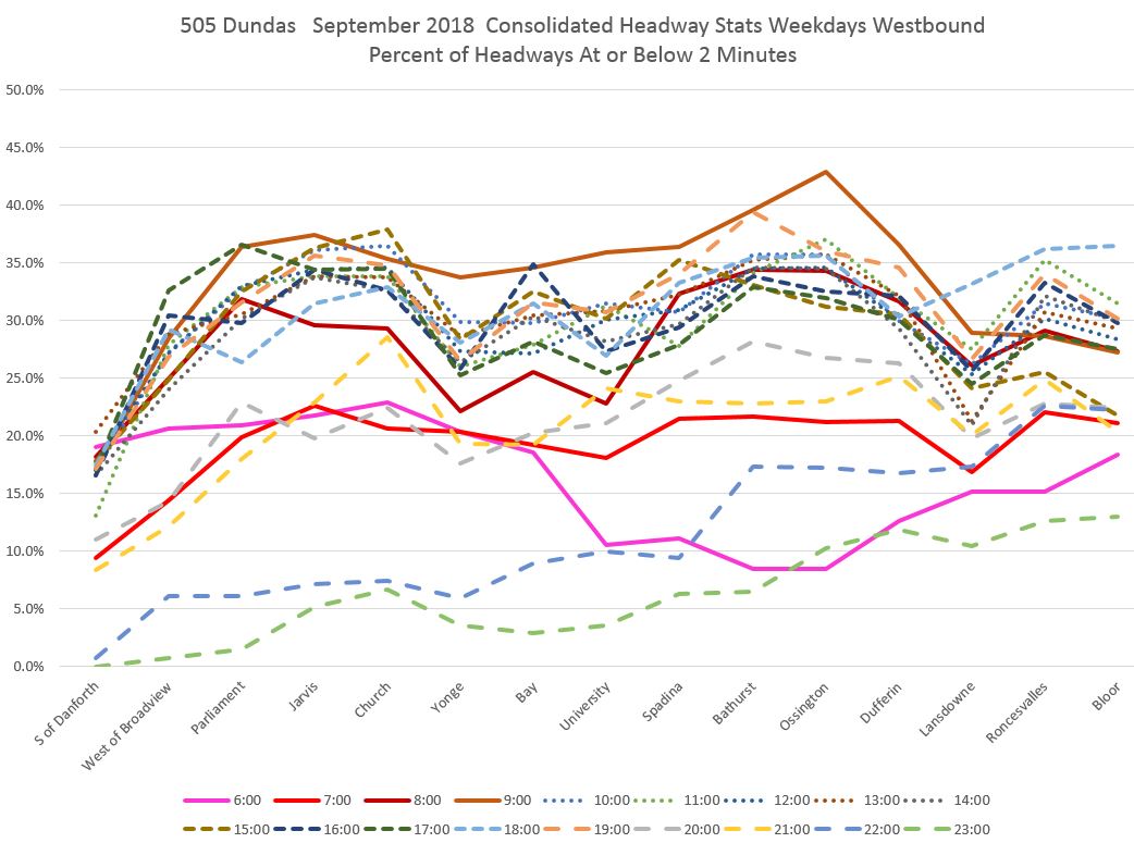
For the AM peak, the lowest proportion of vehicles on close headways lies in the hour from 6-7 am, and it rises to about 35% by the end of the peak period. Note how the values are low at Broadview and Danforth, rise at Dundas and Broadview and then stay fairly consistent from there westward.

In the midday, there is almost no difference on an hour-by-hour basis including, consistently, a slight improvement westbound from Yonge (probably triggered by loading delays and traffic signal timing) that declines as service moves west to Bathurst.

The PM Peak continues the pattern.

In the evening, the highest values are for the hour from 7-8 pm (19:00) and these gradually fall, especially after 10 pm when the scheduled service is less frequent and with that the opportunities for bunching. Note, however, how the same pattern of increased bunching does occur late in the evening, but simply takes longer (Bathurst westward) to really take hold.

Three-D Charts
Another suggestion I received was to plot the data in 3D. This allows the information to be consolidated on a single image, but in the process creates a busier view where some of the detail is not as easy to make out.
In the first example, each slice of the chart represents a location from east to west (front to back) along the route with the times running across. I have tilted the whole display considerably so that the peaks and valleys are visible, but this brings up a problem with this type of chart. If values on front layers are high, they can obscure the back layers. This is a particular problem if service at the outer end of the line is less frequent and therefore the 2-minute percentages are lower.

Here is the same plot with locations along the x-axis and slices of time from front to back. Again there is a need to tilt the display so that the relatively lower late-night values are not hidden by daytime data. Even with the rotation I have used, this problem is quite evident below.

Clustered Column Charts of Headways by Hour
The charts which show all of the headway ranges (in two minute increments) stacked side by side for each hour at a single location have the disadvantage of showing only that location, and requiring that readers switch back and forth between busy charts to see how or if the data change from one to the other. The use of two minute ranges for the data was a tradeoff between granularity and space. Using one minute intervals doubles the width of each hour’s columns in the chart without revealing much more about where the peak value lies. Using three (or greater) minute ranges bring on the same problem with TTC’s own standards, namely that a wide grouping can mask behaviour at a level riders notice.
I will not include the clustered column charts in future articles.
Stacked Columns and Area Charts of Headways by Hour
In past analyses, I have looked at using stacked column charts, but that was short-lived as they tend to be visually busy with the pattern getting in the way of understanding. An area chart shows the same data with the only difference being that the vertical segments are smoothed together. (Note that because the values are percentages, they will always fill the chart to the 100% line regardless of how many actual vehicle headways contribute to the stats.)
One issue with this chart, as some have pointed out in other comments, is that there is a difference between an absolute range of headways as shown by a colour or a line, and a “good-better-best-horrible” scale that adapts to the target level of headways. For example, the dark blue ten-twelve minute band in the chart below is “very bad” territory when the scheduled service is every five minutes or better, but not quiet so bad late in the evening when, the scheduled service might be every 10 minutes.
The chart below shows the bands of headway data as percentages over time. A good deal of the headway values do not lie in the 4-6 minute range of headways scheduled over the day). The darker colours are easy to understand late at night when scheduled headways are wider.
This chart is “messy” in a few ways:
- What is “good” is not immediately obvious because there is no reference line for the target (scheduled) headway.
- The chart shows only one location requiring a reader to flip back and forth between multiple charts to see how values evolve along the route.

The same data plotted as a stacked area chart gets even messier. It’s a nice piece of abstract art, but the pattern gets in the way of understanding the details.

Finally, the raw counts of vehicles observed by hour show how this varies over the day whereas the charts above show the percentage of vehicles in each band. Note that this is the 19-day total.

I don’t like any of the charts above because, like the clustered column charts in the original article, they require multiple pages to display data over the length of a route, and the “artistic” nature of the charts gets in the way of understanding.
Box and Whisker Charts
This type of chart divides the data into four quartiles with emphasis on the two middle ones (corresponding to the percentiles from 25 to 75). This approach can hide information because it gives relatively little information about the spread of values, especially the outliers at the minima and maxima. In a month’s data, there is bound to be at least one bus running in an extremely short headway, and one on an extremely long one. This pulls the “whiskers” to the outer reaches of the chart without any indication of how common events in this range can be.
The charts below show the data for the four hours between 6 and 10 am in September, westbound on 505 Dundas, in Box and Whisker format. The y-axis maxima are set to 20 minutes so that the charts can be directly compared, but this clips instances where the maximum values lie above that level.
Each column displays the range of values in quartiles:
- The bottom “tail” shows the range of values from the minimum to the 25th percentile.
- The lower box shows the range of values from the 25th to the 50th percentile.
- The upper box shows the range of values from the 50th to the 75th percentile.
- The top “tail” shows the range of values from the 75th percentile to the maximum.
One big problem immediately pops out: the length of the tails. Over the course of a month’s data for one hour’s operation, there will always be at least one long gap. That’s pretty much par for the course on a transit route. That pushes the maxima out to high values that should not be read to imply an equal distribution of headways over the range that the tail covers. In fact, most of the values are closer to the bottom of that range, but this is masked by this type of chart. Similarly, there will always be at least one pair of buses running back-to-back and this will cause a uniform minimum value at or very close to zero. Again, this does not reveal the distribution of headways within the band.
The boxes show a range of headways that occurred 50% of the time while the tails show the other 50%. Ideally, the tails should be short, but generally speaking they are not.

As we progress hour by hour, the central boxes get wider indicating that half of the trips lie within a wider range of values (25th to 75th percentile). However, the top tails also grow off of the edge of the charts. By 9:00 every location has a maximum above the 20 minute line.


The chart below shows the 9:00 data with the y-axis adjusted so that the tops of each column are visible. Yes, this means that on at least one day, there was a gap of over 25 minutes that travelled the width of the route.

Here is the service chart for Tuesday, September 4, 2018 when these extreme values occurred. Note that there is almost no short-turning in an attempt to fill the gaps. The drop in the maximum value charted above was caused by one bus turning back from Parliament Street just before 9:30 am.
This is an example of how consolidating data can give misleading values when there are some outliers such as the situation shown below.

I can see a use for box-and-whisker format in some of the other headway and link time charts I produce, but at a more fine-grained level than an entire month’s data. I will explore this in a further update.
Chart Sets as PDFs
Here are complete sets of the charts used above in PDF format.
Updated October 11, 2018
This update presents a set of charts consolidating various requests into one format. There is an inevitable tradeoff here between complexity and content, and I hope that this finds a reasonable balance.
As I noted in the previous update, “box and whisker” charts run into problems in presenting headways in that for one month’s data, there will always be at least one pair of buses running together, and hence a minimum value at or close to zero. This doesn’t tell us anything. Similarly, there will usually be at least one bus running on a very wide headway thanks to a gap, and this will pull the maximum value well above the more typical headways riders encounter.
To correct for this, I have produced a modified version of the box and whisker format that shows how wide (or not) the outer region of the headway distributions are by including markers at the 10th and 90th percentile points. The chart below (click for a larger version) has the Y (time) axis capped at 60 minutes so that the full length of the “whiskers” is evident.

The next chart shows the same data, but with the Y axis capped at 20 minutes so that the important details are more obvious.
Each horizontal section of the chart presents one hour’s data. Within this each column shows data for individual screenlines along the route. The colour of the column segments indicates the range of values with the middle quartiles showing as wide boxes.
- Red: The lower 10th percentile of values lies within this band.
- Orange: The 10th-25th percentile lies within this band.
- Together these bands comprise the lower “tail” of the chart. One quarter of all headways observed within the hour at the location in the legend fall within this range.
- Yellow: The 2nd quartile, or the range of 25-50% of headways.
- Green: The 3rd quartile, or the range of 50-75% of headways.
- These two bands are the “box” of the chart and show the headways observed half of the time at each time and location.
- Blue: The 75th-90th percentile lies within this band.
- Purple: The upper 10th percentile, 90th-100th, lies within this band. These are the worst of the worst cases.
- These two bands comprise the upper “tail” and account for the final quarter of all observed headways.

This is the chart for the afternoon period from noon to 6:00 pm:

This is the chart for the evening period from 6:00 pm to midnight.

Several notes about these charts:
- A rider at a specific location and time will encounter a range of headways covered by the yellow and green sections of the chart 50% of the time. A further 30% of the time the range will extend up or down to the marker on the “whiskers”, and the remaining 10% of headways will lie in the outer range of the columns.
- Wait times would be half of the headway, on average, assuming would-be riders arrive at stops randomly during the period between buses.
- Note that in many cases, the yellow box has a higher value at Broadview & Danforth than further west on the route. especially during the evening period. This is caused by the tendency of buses to catch up to each other and run in pairs. the top of the green box also rises showing the offset in wider gaps that occurs when more vehicles run close together. The bottom of the yellow boxes routinely protrudes below the two minute line indicating that more than 25% of the trips are operating on short headways.
- The band of headways covered by the two middle quartiles (yellow and green) generally cover a range of 4-6 minutes. This is within the TTC’s “on time” service standard most of the day, but many riders do not receive the frequency of service the schedule implies that they should get.
- Far more riders are affected by the wider headways than the short ones because more riders accumulate during the gap and have longer waits. They are also more likely to suffer from the “where is my bus” problem because the next bus is more likely to be too far away to be seen.
As a specific example, for someone wishing to board westbound at Spadina in the hour between 3:00 and 4:00 pm (15:00 in the chart legend):
- Half of the buses will arrive on a headway between 1 and 6 minutes (yellow and green boxes).
- 15% of the time, the buses will be up to 11 minutes apart and a further 10% of the time they will be even more widely spaced (blue and purple lines above the boxes).
Waiting times will be half of the spacing between buses, assuming the rider can board the first one that shows up.
I believe that this format has consolidated most of the items various commentators flagged. I plan to use the following formats in upcoming articles:
- Average and Standard Deviation charts by location and time to show the degree to which these values vary on a route, if at all.
- Charts of the proportion of service running on a two minute headway or less.
- The consolidated charts of headway ranges by time and location.
Each of these displays different information and suits a different audience.
The set of six charts in the new format is in the PDF linked here:
Many thanks to all who left comments. This process has also triggered the generation of a revised set of travel time charts which will appear in an update to the September review of data for the King Pilot.

And at the terminals, the buses and streetcars should wait at the loading bay, not in the parking bay. Let the passengers sit down in the vehicles, and actually leave on time.
LikeLike
Hi Steve – thanks for the interesting post. Would you consider linking to one data set for a chart that people could play with if so inclined? I have a few ideas but normally I would try to make them on my own rather than waste your time seeing if hey’re any good.
1. For any chart, consider providing a set of reference charts which visually display “ideal”, “good”, and “bad”. For the 505’s consolidated headway bar chart, that would be I guess all yellow and green, then mostly yellow and green with orange and blue rising, then the inverse with very little “correct headway”. The charts make sense to me but I suspect the learning curve on all this stuff could be improved with a reference version shown above, even in small size – perhaps show three versions of the same four hour block.
2. Another idea that came to mind for the headways bar charts was an area chart, showing how as time passes the poor headways take over the route capacity? (like this: https://documentation.sisense.com/Resources/Images/7-2/areastacked.png ) I’m imagining custom colours so that it functions like a topographical map, with good headways in one colour and bad (bunches AND gaps) in the other colours. (i.e. red orange yellow green yellow orange red)
3. Or a stacked area chart, allowing you to look at only one of the headway bands (the ideal headway) but stack multiple locations, which gives the degradation of service as you progress across the city. (like this: https://datavizproject.com/wp-content/uploads/2017/09/DVP_101_200-42.png )
I hope these are helpful to think about at least, if possibly too complex to create in a reasonable timeframe.
Cameron
LikeLike
I’ve long had trouble reading these charts at a glance.
One idea would be to group the headways into buckets (0-3 minutes, 3-6 minutes, 6-9 minutes, 9-12 minutes, 12+ minutes), count the incidence of each in a day, and then graph it so the buckets are on the x-axis and the counts are on the y-axis.
Steve: The data are already grouped into buckets two minutes wide e.g. 0-2, 2-4, etc. The problem with your proposal is that bringing it down to daily counts makes the data meaningless as there are variations from hour to hour. Personally, I prefer the versions with the lines, one for each location, to the bars, but presented the bar version to show what I started out with. The lines show only the under 2 minute headway data and thereby allow consolidation onto a single page for an entire day.
LikeLike
Back when I took a look at graphing this stuff one of the useful ideas was just looking at a routes effective number of vehicles at each time division and graphing…
If 2 or more vehicles are closer than a certain threshold (say 2 minutes on a scheduled 10 minute headway route) then treat all of those vehicles as 1 vehicle for each given time period.
So we get some like:
– 10am – 10 operating, 7 effective (3 bunched)
– 10:01am – 10 operating, 8 effective (2 bunched)
Repeat for all time periods and directions and graph…on long routes or routes that contain multiple branches or multiple routes you can split it up and have some more numbers:
– 10 scheduled (by design), 9 scheduled (by service being operated), 7 in zone, 3 effective
Steve: I will look at this type of analysis in a future update, but like the idea. In effect, consider vehicles that run at close to a zero headway as “not present”. However, this does not work for very frequent routes where the real problem is the very wide headways where they should not exist.
LikeLike
The ultimate problem is: On a frequent service route, I should not be waiting long for a vehicle.
With that in mind, I actually don’t care about the bunching (although that may be the root cause), I care about gaps in service. For this reason I think the bar charts are the best option. It is probably more work, so maybe limit the locations that this data is shown, but I believe it communicates the desired data the best.
Average Headways: I think this is the least useful due to the smoothing out of the data and the possible bias due to skewing.
For the bar charts, I would also opt for a different color scheme to assist in differentiation between the bars. Adding patterns into the mix can help with visual accessibility.
LikeLike
Standard deviation is statistically meaningful in that it shows how well service is managed, but I agree that the “fraction of headways below two minutes” is simpler and better captures customer frustration at bunching. You might even generalize it to “fraction of headways below 1/nth of the scheduled headway” to compare routes to one another.
When both geographical and chronological info are in play (e.g. particular places on a route at particular times during the day) it’d be interesting to see the data displayed as an animated map — overlay a line on Google Maps showing the route, colour code it to represent the severity of bunching, and animate it to represent different times during the day.
LikeLike
On the bar graphs, could you make them feel less busy by consolidating some of the headway values and having fewer bars? E.g. go with 3-minute spans rather than 2, make the top one 10+ rather than 12+, or combining two or more of the middle values (since folks care less if headways are slightly more or slightly less than advertised). I know this is a step towards the problem with TTC’s service stats, but there’s a chance it might help.
The line graphs are still busy, but I don’t know if it will be possible to un-busy them without cutting a lot of useful information.
I don’t know if this would be any better, but how about using stops for the x axis and having different lines for different times of day? Would that make it feel less busy at all? Just spitballing.
I like the standard deviation graphs, but using standard deviation might detract from the accessibility of the information to less data-inclined folks.
Steve: As you will see from my update, I plan to drop the bar graphs as the format obscures more than it shows. Moving to wider spans brings problems because for headways under 10 minutes, too many data points fall into one bucket. When I originally tried this out with one minute graduations, there was more detail in behaviour of the peaks, but also twice as much clutter. Two minutes is a compromise.
LikeLike
Perhaps box and whisker plots comparing different routes work better visually to compare consolidated actual headways between different routes to highlight how some are much more unreliable?
LikeLike
From a rider’s perspective, people care about the big gaps more than the small ones (even though they tend to be opposite sides of the same coin).
What about having a stacked bar graph for each major stop location, with percentage of service that is in each 2-minute bucket? So you might have “More than 1 min. early” (or “Less than 1 min. since last bus”), “1 min. early to 1 min. late”, “2-3 min. late”, “4-5 min. late”, and “5+ min. late”.
This would give a good visual of how people experience the headways rather than averaging things out (current KPI) or a standard deviation (which just says what a ‘normal’ range off the average is, without showing how the deviations break out).
Steve: I prefer the short headways as a bellweather because they are not as subject to skewing from the occasional very high value (see the discussion under “box and whisker charts”) that would have to be filtered (begging the question of what should be filtered and what should be left in). Also, the concept of “late” is meaningless. Headways should be measured against a target value, not against the schedule (ie late or early arrivals) except in cases where headways are wide enough that the schedule really matters (generally above 10 minutes). Also, I am not much of a fan of the stacked bar graphs.
LikeLike
Thanks for the analysis Steve. Between the GPS units on the vehicles and real time traffic data you would think it would be pretty easy to determine when headways are off due to unavoidable conditions, and when they are caused by drivers with a poor sense of obligation to ridership and the system’s overall reliability, and to staff vehicles accordingly.
Re: “And at the terminals, the buses and streetcars should wait at the loading bay, not in the parking bay.”
I have no idea why, but the buses at Gunn’s Road in the stockyards area wait on the road, blocking one lane of traffic instead of in the loop itself. I saw an inspector there overseeing the whole thing. When the first bus pulls out into the left lane to turn east onto St. Clair, the second bus is still in the right lane, so the two buses are pretty much blocking all vehicular traffic. I didn’t see any reason for them to not wait in the loop itself.
LikeLike
This is the thing, like with the upcoming 504A/B spilt this Sunday, we all hope to see streetcars leaving right away, mainly at Dundas West and Broadview stations, where only 1 Flexity can go at a time, but at Dufferin and Distllery Loops is where the operators *should* layover.
LikeLike
I wonder if some relatively simple number(s) can be generated, rather than charts which always seem to require explanations. It seems to me that it’s easier to get people’s attention by giving them a simple, alarming number, and then being able to clearly explain the way the number was generated. The other way, showing a chart or graph, and having to explain why it should alarm viewers, is less effective.
I have a couple of ideas that may produce a simple number.
Determine the actual average headway over, say, an hour (length of time needs to be long enough to get a reasonable number of trips). Calculate percentage of observed headways which are less than 50% of the average, and the percentage of observed headways which are more than 50% of the average. (The 50% may need to be tweaked on one side or another.) Add the percentages together. The total would be percentage of service that’s running bunched. So it may produce a bunching percentage, like “during the day, there’s 55% bunching on Dundas”.
An alternate way to generate a number is to determine the ratios between the shortest headways and the longest headways. So if the two shortest headways are 1 minute, and the two longest headways are 15 minutes, then the “bunching index” would be 15, which should scare anyone, since if the line was running properly, the bunching index would be 1, and 15 is obviously much, much greater than 1.
Steve: I am contemplating an analysis that uses the average headway as a starting point and then works out from there in “good”, “bad” “horrible” quality measures. As I have remarked elsewhere, there will ALWAYS be some very short headways and some very long ones (the minima and maxima within a specific hour for the month) and these numbers are almost meaningless. What is more important is the distribution of values outside of a range we might call “good”. If only 1 instance of a 40 minute gap occurs in a month’s data, then this really does not tell us anything about “typical” service.
LikeLike
I think these might be better reimagined as box-and-whisker plots, which are informationally denser. They’re a little unfamiliar to people, though, so they might require some training in how to read.
Steve: They might be informationally “denser”, but actually mask important details. See the update in the article.
LikeLike
On the charts could you add a “target” or “scheduled service” line on the graphs to show what the “ideal” service timing for the route at these points should be?
LikeLike
I am also interested in what comments people have because I am hoping to use the data collected by TransSee to dynamically generate similar reports for, not just the TTC, but for the other agencies supported by TransSee.
I think to focus should be on the long headways rather then the short, since that’s what actually what causes people problems, even if it is a bit harder to measure.
LikeLike
Your route analyses are an amazing resource with a great deal of raw data but, I think, that even for transit aficionados, they are somewhat overwhelming. As you say “Riders do not care if a bus or streetcar is “on time” on many routes, only that they show up regularly.”
While there is a risk to over-simplify data (matching the TTC’s idea that ‘on time’ is + or – 5 minutes) but I wonder if it would be clearer to use your full data and select a few stops on a route and chart how long a customer arriving at them would wait for the next vehicle and do this at 6 – 8 standard times each day, every day. The number of stops ‘charted’ would depend on the length of the route but would, I think, include either the departure point or the first stop after it, the last stop before or at the terminus point and, on a route like King, maybe 5 or 6 in between. I would then look at maybe 6-8 specific hours. One before am rush, one during it, one in mid-morning, one in mid-afternoon, one at pm rush and one in mid-evening and one late at night. Doing this would allow a ‘casual reader’ to look at ‘their route’ and see that if they were at King & Jarvis at 8pm (for example) the normal wait time on a weekday would be x minutes. This would, I think, flag problem areas/times/routes and then the full data-set could be analysed in greater detail.
Good luck, it is hard to see a ‘perfect’ way to do this but this might be one to consider, at least as an experiment.
LikeLike
Here is what is important about headways to me, and I presume many other people.
In the AM rush, my employer (before I retired) had an expectation that I would arrive at work on time. Yet, everyone also knew that, this being the TTC, bad stuff happens that makes everyone late. So the tolerance level was about one late arrival per month. Since I worked Monday to Friday, that was about 20 working days per month. So a 95% on-time arrival rate was expected at my workplace.
So the fundamental question is: How long is the TTC trip for 95% of the time? In other words, if I were to take all the times for my TTC trip during the AM rush and drop the worst 5%, what is now the longest time? Because that is the amount of time that I have to allow for my trip in order to arrive at work on-time 95% of the time.
With regards to the headways, the same methodology applies to the AM rush. When I show up at a TTC stop, what is the maximum time that I will have to wait 95% of the time? In other words, “average” headway does not matter. What matters to me is how much time I have to allow waiting for a TTC vehicle in order to arrive on-time at work 95% of the time.
A totally different logic applies to the PM rush. In the AM rush, the key question for me is, “What time do I have to leave home at in order to arrive at work on-time 95% of the time?” But in the PM rush, the time to leave the workplace is not chosen by me but by my employer. And my wife and children do not expect me to be home at a fixed time.
However, there is a certain life dissatisfaction when the TTC is late getting me home from work. My wife and children grow to expect me home at a certain time. If the TTC makes me late for dinner, there is an unhappy family. I will define this late dinner/family unhappiness time as being 15 minutes later than the average travel time. So in the PM rush, the question is, “What percentage of the time will the TTC get me home 15 minutes longer than average?”
For me, those are the key measurements of TTC performance.
Steve: That is a very difficult question to ask for any specific commuter because the potential variability in travel time depends on the routes used and the time of day. This is a place where management metrics fall apart because of the compounding effects of each route, not to mention your cumulative experience.
As a simple example, it is not uncommon to see performance goals of 90% or even 95% (leaving aside the obvious question “90% of what”). If, say, there is a goal that there should not be a major screwup on the subway 95% of the time, do we mean on the network as whole, or does the target apply to each line separately (that’s how they are reported by TTC).
If you only travel on one line, the probability of not getting caught by a screwup “today” is 95%, but then 95% again for tomorrow, and so on. It takes 14 days for the cumulative probability to fall below 50%. If you are counting on both lines working (and we won’t even mention the RT), then of course you get to 50% in 7 days while management still gets a gold star. 95% is probably far too generous for current conditions, and so you are likely to encounter a big cock-up often enough that it will be the event you dread every day. And we haven’t even transferred to a bus or streetcar line yet.
At one point the TTC was looking at “journey time metrics” that would track a bundle of standard trips through the network based on actual conditions on the routes. I suspect they found a huge fluctuation in travel times that could not be translated into a metric management could pat themselves on the back for. “Fixing” that type of problem also requires a system-wide approach to service quality, not simple fixes here and there. The journey time metrics never saw the light of day.
LikeLike
Steve, I am wondering if it might be more understandable for a general audience if, where it is reasonable, the horizontal axis is utilized to identify the set of timed stops. With the addition of a second vertical axis, it may be possible to demonstrate the same results to the reader, while capturing the entire route, instead of one point or one section.
LikeLike
Finding clear ways to present the data is obviously a huge challenge. I’ll try to think about it more. For now.. I think wait times are a better metric to be charting than headways.
First, from a purely linguistic point of view, I think riders are more likely interested in wait times than headways.
I also think it is statistically more useful to look at wait times. For one, there is the Bus Waiting Paradox. That’s further complicated by what I see as a preference of (some?) TTC drivers: they actively try to run behind a buddy, because it means fewer passenger interactions, which I guess they see as less work.
Finally, I think a chart of Expected Wait Time vs. Hour of the Day ends up being more readable than the current Consolidated Headway Stats charts. There wouldn’t be a need for binning on a bar chart, it could just be a line. Possibly two lines, with ideal wait time (aka Average Headway), and measured expected wait time on the same axis.
So, I really prefer the Expected Wait Time model you were working on in this post (although I guess I’d suggest a shorter interval (10 seconds instead of 1 minute?).
I guess there must be a reason why you tried and dropped it? Even just as a one time thing, an effort at putting expected wait time on the same graph as headways, just to see how they differ, would be an interesting exercise.
Steve: Yes, as the discussion (now much extended) in the article indicates, there are a lot of challenges in quantifying service quality, and in this round I homed in on the two-minute line (bunched service) rather than trying to merge all of the headways together. To the degree that service is bunched, it is not providing the advertised level of convenience and probably sees more vehicles on the leading “gap” buses and streetcars than on their followers. Average rider experience is worse than that claimed by TTC’s published schedules or average loads.
I am still contemplating how to build a display that will dynamically adjust to “target” or at least to average values over route segments and times of the day.
LikeLike
You’ve done a lot of work here Steve (which is, needless to say, as always, very admirable), but I think the charts are not immediately intuitive and would require some effort in examining the different metrics (average headway, standard deviation, etc.) in detail to get the whole picture.
On the other hand, “bunching” is a phenomenon which is very easy to intuitively grasp when you see it. I think the easiest way to communicate the problem would be to create some sort of “bunching index” from the data you have presented here. I have not invented a formula, but I think it would involve the standard deviation and the headway distribution (your colourful bar charts). I don’t know if average headway would be useful in this regard.
This would be normalized on a scale, assume for now it to be from 0 to 10, so let’s say if we have a route where we should see 5 vehicles in the space of 15 minutes, if they come 5 minutes apart the bunching index value would be zero (no bunching), but if the spacing between them is zero minutes the value would be 10 (total bunching). The normalized scale idea works, since this is very easily defined concept on the extremes: either the service is evenly spaced as it should be, and thus there is no bunching, or all the buses are coming right after one another, trailing each other, which means you have total bunching. Of course, this is clearly defined within a given interval; say a quarter, half, or full hour – if we analyzed an entire day, “total bunching” would mean that all the day’s scheduled departues from a terminal leave right in the morning one after the other, which obviously never happens. You would know better than I what to take as the unit of account (an hour, or shorter?).
I think here you’ve already done all the hard work, and if you could figure out just the proper formula for an index, it would be easy to calculate in your spreadsheets.
LikeLike
Here’s an idea related to the above:
Let’s say we are supposed to have on a route three departures per hour. Ideal spacing, no bunching, means that the headway should be 20 minutes between each bus. So buses leave at say :00, :20, and :40 from the terminals, and keep their spacing even throughout the route.
Extreme or total bunching means all three buses leave at the top of the hour, trailing each other, and then you have to wait for 60 minutes until the next three buses come. So we have headways of 0, 0, and 60.
Basically, bunching creates a large number of small headways and a small number of very large headways. Thus, the most useful thing to compare is the maximum and minimum headway.
In the ideal case, both are 20, and the difference is zero, which gives our no bunching value on the normalized scale.
In the extreme case, this difference is 60, so to get that to 1, we divide by the product of the ideal headway (20) and the number of buses (3). Multiply by 10 to get a scale from 0 to 10.
Let’s say we have a less extreme but nonetheless signigicant bunching, where the headways are 5, 10, and 45 minutes. The index would be 40/60 * 10 = 6.67.
Let’s say it’s milder with headways of 10, 15, and 35 minutes. The index is now 25/60 * 10 = 4.17.
I’m sure more thought needs to be put into this, but perhaps it’s a start.
Another approach might be to tabulate the % difference between sucessive headways and take an average. In the ideal case above, it is zero. Bunching will create a huge % change (usually way over 100%) which will skew this average towards a large number. This would take into account all of the spacings, not just the min. and the max.
Steve: As I have mentioned in other replies, I still have to figure out a way to dynamically adjust what appears as a target “good” headway to the actual service level at each location and time. One thing that I really have to avoid is a scheme that is too formula-bound in the sense that it produces a number that as to be explained rather than one that is intuitively obvious. The other challenge, of course, is to avoid a metric that is so tied to “averages” that it misses the quite numerous occasions fare removed from the average that bedevil riders in the real world.
LikeLike
I find all of these graphs sort of opaque. They show so much data that it’s too hard to interpret. The data should be simplified to the point where it clearly shows the message that you want to convey.
I think it would be better to show it as “how long do I have to wait for the bus/train?” There should be three lines showing the 10th, 50th, and 90th percentile of wait times for the next bus. Then it will be easy to see: at around 5pm, you usually have to wait 5 minutes for a streetcar, but sometimes it’s 30 seconds, and other times it’s 30 minutes.
Steve: See the updated article in the section on “box and whisker” plots.
LikeLike
Another issue is that the data is shown by vehicle and not by passenger. If vehicles are bunched together and come one minute apart, then only one minute of passengers will benefit from the short headway. If there is a bus that’s 10 minutes late, then 10 minutes worth of passengers will end up waiting at the bus stop, they’ll all have to wait longer, and they’ll all have to cram on the bus. So even though it’s only one bus with a longer headway, more passengers will be disproportionately affected by that one bus because more passengers will end up waiting around during that longer headway.
Maybe you can have an assumption that passengers arrive at a constant rate during a one hour period, then you can classify passengers as happy (short wait), neutral (normal wait), dissatisfied (long wait), angry (very long wait). Then you can just draw little coloured happy/sad faces, and it’ll be easier to see the scale of headway problems in terms of affected passengers.
LikeLike
Sorry, can’t stop thinking about this. I guess a percentile graph of wait times, per passenger is maybe the way to go then? The more I think about it, the more I think per vehicle time doesn’t capture the passenger experience correctly. If there are 10 buses that come all bunch together in the first 10 minutes, and then the next bus is in 50 minutes, then that one late bus must be weighted more because 5x more passengers will end up taking that late bus than those 10 buses that came 1 minute apart. Of course, in those 50 minutes, some will end up waiting for 50 minutes, some for 40 minutes, some for 20 minutes, and some for only five minutes. So you have to capture that correctly in the math/modelling.
LikeLike
So even for the first graph, where you show the headways of vehicles on a specific day, you should graph it like this in order to capture the passenger experience of headways.
It you arrive at 9:00, you have to wait 15 min for the bus. If you arrive at 9:05, then you have to wait 10 minutes. If you arrive at 9:16, you only have to wait one minute. Those short headways only benefit a small number of people, but the long headways both affect more people and affect them a lot more.
Steve: The services I am looking at run much more frequently than quarter-hourly. The problem is that “frequent” services often are not because of bunching and gapping. Also, the exact time these gaps might occur is not predictable at the granularity your example implies.
LikeLike
Not to be argumentative Steve, but..
You are exactly describing the Bus Waiting Paradox. The expected wait time for a bus is always higher than half the headway. In fact, in the Bus Waiting Paradox, the assumption is that bus arrivals follow a Poisson distribution; counter intuitively, the result is expected waiting times equal the full headway, not half the headway.
So, rather than being a weakness, expected wait times actually deal with the 1-9-1-9 problem very well.
On other topics..
It’s clear that in fact there are three important numbers for either wait or headway graphs. The long term schedule, the deployed vehicles (accounting for short turns, breakdowns, whatever else), and the actual measured times.
I like the whisker charts.
Thanks so much for the enormous time and effort you put into this stuff!
Steve: I may try the whisker charts for travel times as there tend to be fewer instances of really wildly off the mark values in that data. For headways, one can always count on an almost zero value, and on the span of a month, at least one very large value is fairly common.
And, you’re welcome! I am trying to concoct a “standard” format that I can simply populate every time I have data for a new route/month, and with charts that address various commonly asked questions.
LikeLike
Personally, I find the bar charts hard to understand. I haven’t figured out a better chart-style alternative, however. But what about this? “Equivalent headway”:
(∑ h_i^2) / (∑ h_i)
That is, the sum of the squares of the headways, divided by the sum of the headways. A bit unintuitive at first, but consider these mathematical facts:
1) If the headways are all equal this is just the headway. The idea of this measurement is to take a complex set of headways and boil them down to an equivalent equal headway.
2) Adding another vehicle right on top of another doesn’t change the equivalent headway at all. This means adding an h_i which is 0, which makes no difference to either sum. This is correct, because completely bunched vehicles don’t help with headway.
3) I don’t consider capacity; I assume all waiting passengers can load. Bunched vehicles can help with capacity, although if ridership is so high that bunched vehicles are needed, it’s probably better to join them mechanically and use some sort of rail system to guide them.
4) Consider slightly bunched service, say alternating 3 and 7 minute headway. This is (3^2 + 7^2) / (3 + 7) = 58 / 10 = 5.8 minutes. While one could quibble about the exact number, clearly service that alternates between two headways is better than service at the longer headway but worse than service at the shorter headway, and also slightly (but not much) worse than even service on the same frequency (12 vehicles per hour in this case, or 5 minute uniform headway).
5) Now consider a long gap followed by even service (remember I’m not worrying about capacity). Let’s say 1 hour gap followed by n vehicles in the next hour. This is (60^2 + n*(60/n)^2) / (60 + n*(60/n)) = 30 + 30 / n. If n is 1 that is just 60 or the correct 1 hour headway. If n is 6 that is 33 or a 33 minute equivalent; considering that half the people wait up to an hour and the other half wait up to 10 minutes that seems like it might be right. If n is infinity it is just 30 which makes sense: half the people wait an hour and the other all board immediately.
6) The schedule, either with fixed arrival times or a planned headway, is not an input into this calculation. It does implicitly assume frequent service on a planned headway, because with fixed arrival times people will attempt to meet the scheduled time. So we can just ask “how good is the service as operated?” without worrying about which routes are running more or less service than initially promised. In particular it might turn out that some routes with “4 minute service” but bad bunching aren’t actually providing better service than routes with “6 minute service” but actually holding reasonably close to planned headway.
7) One more example, from a previous commenter: 10 buses once a minute, followed by a 50 minutes gap: (10 * 1^2 + 50^2) / 60 = 2510 / 60 = 41.8. This seems reasonable; a small but noticeable group of people got excellent service, but then a substantial majority waited an average of 25 minutes in a 50 minute gap in service. Better than 50 minute service all the time, but not really by all that much.
Now that we’ve reduced service down to a single number, we can more easily make a chart that covers different times of the day. Simply break the day into blocks of an hour or two and calculate the equivalent headway for each period. Then graph this as a bar chart.
I have glossed over two issues: what happens at the beginning and end of the period? At the beginning it’s easy: the first headway is the time between the beginning of the period and the first vehicle showing up. Any vehicle that arrives before the beginning of the period does not count because it doesn’t help passengers who arrive during the period. At the end it’s a bit tricky: what to do if there isn’t a vehicle right at the end of the period? I think the answer has to be to go to the first vehicle after the planned end of the period because that is the vehicle which will pick up passengers arriving at the end. However, the portion of the headway that is after the end of the period should be subtracted out. So the formula becomes:
((∑ h_i^2) – w^2) / ((∑ h_i) – w)
where w is the waiting time after the end of the period to the arrival of the next vehicle.
I think the big benefit here is that this number is not some made-up scale or assessment result in an arbitrary range; it’s simply a period of time, expressed in minutes or seconds or whatever, which appropriately reflects the overall effect of the service as experienced by riders.
The next step would be to weight by how busy the route or system is at different times of day. This would allow generating an overall number that would reflect the experience of riders as a group; bad service at rush hour has a much bigger impact overall than in the middle of the night (although not necessarily a bigger impact on the rider who is harmed by the bad service).
Steve: I have been down this road before.
First, note how your calculation of an effective headway translates alternating 3 and 7 minute headways to 5.8 minutes versus an average of 5. That’s not much of a change, but the problem is that it takes no account of the fact that most riders will be served by the 7 minute bus which will also be more crowded. Indeed that crowding will contribute to slower operation and the 3 minute bus will quickly catch up making this a 9/1 or 10/0 situation for headways. This is also part of the danger of measurement only at terminals as the TTC does.
Someone might be tempted to say that an “effective” headway of 5.8 isn’t much worse that one of 5.0, but try telling that to riders. One thing we know from transit research is that the perception of wait time is non-linear. Very short waits, especially if a vehicle is physically in sight, don’t “feel” bad at all because the bus is “here”. The longer a wait gets, the greater the “will my bus ever show up” feeling mounts compounded with “will I even be able to get on”.
Another point is that calculating an index in “minutes” does not get around the fact that this is an abstraction, not real time.
I really prefer not to concoct some sort of index or metric that does not directly report what is happening because this adds a layer of interpretation and a bias toward whatever assumptions are in the formula. People can easily understand averages, and they can understand the concept that “x% of the service will arrive within y minutes”. This is an easy translation from quartiles/percentiles. Of course, “will arrive” has to be qualified by that standard statistical caveat that past behaviour is no guarantee of future conditions. Conditions have to be roughly the same “today” for “yesterday’s” results to predict what a typical rider will see.
LikeLike
This is VERY true and why I suggested providing ‘outline tables’ showing the average time a customer would have to wait for the next vehicle at a few (major) stops if they arrived there at certain (fixed) hours. Though this would not explain the situation, it would, I think, be fairly easily understandable.
LikeLike
Kevin’s comment: I bet I know exactly why. Suppose I take a bus to the subway and then another bus to my final destination. So I use three lines and two transfers. If each line has a 90% on-time record, then the probability that all three will be on-time is 0.9 X 0.9 X 0.9 = 0.729
Similarly, if each line has an 80% on-time record, then the probability that all three will be on-time is down to just a tad over 50%.
Any TTC passenger can attest that real-life TTC trips that involve two transfers will tend to have a wide variability in trip time.
LikeLike
Possibly totally unrelated but I had to go from Brampton to a conference at the Westin Prince hotel on York Mills in the Don Valley. Because I had knee surgery the week before I could not drive so I took the GO train to Toronto, about 50 minutes. I took the subway to York Mills, about 20 minutes but I’m not positive and then the York Mills bus, 12 minutes. The total trip time was under 1.5 hours which was less than the last time I drove it on the 401. I contemplated taking the GO bus to York Mills Station then the 95 which would have been about 20 minutes faster but decided or the scenic rail tour.
LikeLike